tsgarch

1 Introduction

The Generalized Auto-Regressive Conditional Heteroscedasticity (GARCH) model of Bollerslev (1986) and the numerous extensions which have followed since, is a framework for modeling the dynamics of the conditional variance. It has proved particularly popular, particularly among financial market practitioners, but also in other areas were the arrival of unexpected new information may lead to non-instantaneous decay (persistence) and/or asymmetric reaction to good and bad news (news impact).

Many programming languages have one or more implementations of GARCH, with R having no less than 3, including the garch function from the tseries package, fGarch and rugarch. A select R package review is provided in Hill and McCullough (2019), and a cross language package review on asymmetric GARCH in Charles and Darné (2019). The suggestions and constructive feedback in these papers were taken into account when developing this new package, as were many of the user comments over the last 10+ years.

The tsgarch package is a partial re-implementation of rugarch, by the same author, with key differences summarized below:

  • does not (yet) implement all GARCH models in rugarch. FIGARCH, Multiplicative Component GARCH and Realized GARCH are not currently implemented.

  • does not implement joint ARFIMA-GARCH estimation, but does allow for a jointly estimated ARMA(\(p,q\))-X mean equation (see Section Section 2.1) in addition to the constant. With so many options for modelling the conditional mean beyond low order ARMA dynamics, many of which are available in the tsmodels framework, it was decided to keep this package’s mean equation support deliberately limited rather than pursue full joint estimation of arbitrary mean dynamics with the variance equation. For a fully general mean equation (e.g. ARFIMA-X, or higher order fractional dynamics), the 2 step estimation approach, whereby the residuals of the conditional mean are passed to the variance dynamics estimation, remains available and may be more flexible in what can be achieved, even if potentially less efficient for small sized datasets. Additionally, the ARCH-in-mean model is no longer available, as it was found to have very limited value within the tsmodels framework or in general, this author’s experience. The sibling tsarma package remains available for standalone ARMA(p,q)-X modelling outside the GARCH setting.

  • makes use of automatic differentiation (autodiff) during estimation, via the TMB package. This is in line with similar approaches in other models written in the tsmodels framework. Using autodiff allows for more confident estimation and more accurate standard errors. Autodiff is also used for the more complex inequality constraints of some models which involve evaluation of an expectation, in order to generate more accurate Jacobians of these inequalities for use during optimization.

  • adopts a custom approach in optimization using parameter scaling which avoids problems with convergence and numerical stability.

  • fully implements and correctly documents a number of sandwich estimators making use of the sandwich package framework (with methods for bread and estfun and meat/meat_HAC functions).

  • makes use of S3 methods and classes, abandoning the S4 approach of rugarch. Additionally, while making use of standard methods from the stats package, some of the methods are based on those exported from tsmethods, consistent with other packages in the tsmodels framework. The Appendix provides a table with a hierarchical overview of the main functions and methods currently implemented in the package.

  • provides more accurate and informative output, including standard errors, confidence intervals, and a more detailed summary output including a fancy flextable output for the summary method.

  • provides numerous fixes and enhancements to the original rugarch code, including the unconditional variance of the exponential GARCH(1,1) model, and better startup conditions for the initialization of the recursion.

  • provides more extensive documentation and high coverage of unit tests, with a focus on the accuracy of the estimation and the correctness of the output as well as catching many corner cases.

This vignette provides a mathematical summary of each type of GARCH model used, general assumptions regarding initialization and other estimation details as well as the forecast equation. Separate vignettes are available with code demonstrations.

2 GARCH Estimation

The density function, based on the distributions available in the tsdistributions package, is expressed in terms of the location, scale, skew and shape parameters \(\left\{\mu_t,\sigma_t,\zeta,\nu\right\}\), normalized to give zero mean and unit variance:

\[ z_t = \frac{y_t - \mu_t}{\sigma_t} \] {#eq:garch_estimation}

where \(\mu_t = E\left(y_t|x_t \right)\) and \(\sigma^2_t = E\left((y_t - \mu_t)^2|x_t\right)\), with \(x_t\) the information set available at the period immediately before time \(t\) and may include both external regressors and lagged values of \(y\). Assuming that the distribution of \(z_t\) is independent of the conditioning information set1, then:

\[ g\left(z_t|\zeta,\nu\right) = \frac{d}{dz}P\left(z_t<z|\zeta,\nu\right) \] {#garch_gfun}

which is related to the distribution of \(y_t\) by through the scale term:

\[ f\left(y_t|\mu_t,\sigma_t,\zeta,\nu\right) = \frac{1}{\sigma_t}g\left(z_t|\zeta,\nu\right) \tag{1}\]

The parameter set \(\theta\), which includes the conditional mean, conditional variance and distributional skew and shape parameters is estimated by minimizing the negative of the log-likelihood:

\[ \theta_{ML} = \underset{\theta}{\operatorname{arg\min}}\sum^T_{t=1}-\mathrm{log}\left(\frac{1}{\sigma_t}g\left(z_t|\zeta,\nu\right)\right) \tag{2}\]

subject to upper and lower parameters bound constraints as well as the persistence constraint (\(P<1\)) and other non-negativity constraints. Estimation is performed using the nloptr solver with analytic Gradient and Jacobian of the constraints2 provided through autodiff in TMB.

2.1 ARMA(X) Mean Equation

By default (arma = c(0,0)) \(\mu_t\) reduces to either zero or a constant \(\mu\) (controlled by the constant argument to garch_modelspec), in which case \(y_t - \mu_t = y_t - \mu\) is simply passed to the conditional variance equation. Setting arma = c(p,q) instead activates a jointly estimated ARMA(\(p,q\)) mean equation:

\[ y_t - \mu = \sum_{i=1}^{p}\phi_i\left(y_{t-i}-\mu\right) + \varepsilon_t + \sum_{j=1}^{q}\theta_j\varepsilon_{t-j} \tag{3}\]

so that \(\mu\) retains its interpretation as the unconditional mean of \(y\). Equivalently, the innovation \(\varepsilon_t\) is obtained recursively as

\[ \varepsilon_t = y_t - \mu_t = \left(y_t-\mu\right) - \sum_{i=1}^{p}\phi_i\left(y_{t-i}-\mu\right) - \sum_{j=1}^{q}\theta_j\varepsilon_{t-j} \tag{4}\]

which only requires \(\varepsilon_{t-1},\ldots,\varepsilon_{t-q}\) from previous time steps, so the whole recursion can be evaluated forward in a single pass once \(\mu\), \(\phi_i\) and \(\theta_j\) are known. Setting arma = c(0,0) (the default) collapses Equation 3 exactly to the pre-1.0.5 constant-mean behavior, \(\varepsilon_t = y_t - \mu\), with no change in results. The constant argument remains independent of arma: it controls only whether \(\mu\) is estimated or fixed at zero.

It is \(\varepsilon_t\) (rather than \(y_t - \mu\)) that is passed on to the conditional variance equation of whichever GARCH flavor is chosen, decomposed as

\[ \varepsilon_t = \sigma_t z_t, \qquad z_t \overset{\textrm{iid}}{\sim} D(0,1;\ldots) \tag{5}\]

with \(\sigma_t\) the conditional standard deviation implied by the chosen GARCH variance equation, and \(z_t\) an iid draw from the chosen conditional distribution \(D\), with any shape/skew parameters estimated jointly with everything else.

The combined pre-sample/burn-in length used to initialize this recursion is \(\max\left(\textrm{GARCH order}, \textrm{ARMA order}\right)\), so that e.g. an ARMA(2,2) mean equation together with a GARCH(1,1) variance equation initializes correctly; over that pre-sample the process is assumed to start at its unconditional mean with zero shocks, i.e. \(y_t = \mu\) and \(\varepsilon_t = 0\).

When arma is active, fitted() returns the (now genuinely time-varying) conditional mean \(\mu_t = \mu + \sum_i\phi_i\left(y_{t-i}-\mu\right) + \sum_j\theta_j\varepsilon_{t-j}\) rather than the constant \(\mu\), and residuals() returns the true ARMA innovations \(\varepsilon_t = y_t - \mu_t\) rather than \(y_t - \mu\). Both predict() and simulate() account for the ARMA dynamics in the mean forecast/simulated paths, and tsfilter() continues the ARMA recursion when incrementally filtering newly appended observations. ARMA support is available for all GARCH flavors described in Section Section 2.9, including igarch and ewma.

2.1.1 Regressors in the Mean Equation

Regressors \(x_{k,t}\) (\(k = 1,\ldots,s\)) can additionally enter the conditional mean, via the xreg argument to garch_modelspec, with coefficients \(\tau_k\) (named tau1, tau2, … in the parmatrix). The xreg_type argument selects between two conventions. The default, xreg_type = "arma_errors", applies the ARMA recursion to the regressor-adjusted deviations:

\[ y_t - \mu - \sum_{k=1}^{s}\tau_k x_{k,t} = \sum_{i=1}^{p}\phi_i\left(y_{t-i} - \mu - \sum_{k=1}^{s}\tau_k x_{k,t-i}\right) + \varepsilon_t + \sum_{j=1}^{q}\theta_j\varepsilon_{t-j} \tag{6}\]

This is the convention of stats::arima(xreg = ) and of the sibling tsarma package: the regressors are filtered by the AR polynomial, \(\tau_k\) is the long-run marginal effect of \(x_{k,t}\) on \(y_t\), and \(E\left[y_t\right] = \mu + \sum_k \tau_k E\left[x_{k,t}\right]\), so \(\mu\) retains its interpretation as the unconditional mean of \(y\) net of the regressor contribution. The alternative, xreg_type = "armax", is the rugarch convention:

\[ y_t = \mu + \sum_{i=1}^{p}\phi_i\left(y_{t-i}-\mu\right) + \sum_{k=1}^{s}\tau_k x_{k,t} + \varepsilon_t + \sum_{j=1}^{q}\theta_j\varepsilon_{t-j} \tag{7}\]

Here the regressors are not filtered by the AR polynomial, so \(\tau_k\) is the impact (contemporaneous) effect and the long-run effect of a sustained change in \(x_{k,t}\) is \(\tau_k/\left(1 - \sum_i \phi_i\right)\). The two conventions differ only by the lagged-regressor term \(\sum_k\tau_k x_{k,t-i}\) inside the AR feedback, and are therefore algebraically identical whenever \(p = 0\); the choice of xreg_type only matters when the mean equation has AR dynamics.3 In both conventions it is again \(\varepsilon_t\) - not \(y_t - \mu\) - that is passed on to the conditional variance equation, exactly as in the pure ARMA case.

xreg must be an xts matrix aligned with y: same number of rows, matching time index, no NA/NaN/Inf values, and full column rank (including against the constant when constant = TRUE) - violations are rejected at specification time. Because the recursion consumes a regressor value at every step, predict() and simulate() require future regressor values (newxreg with h rows, xreg with h + burn rows respectively), and tsfilter() likewise requires newxreg covering the appended observations; if the model was specified with xreg but no future values are supplied, a zero matrix is substituted with a warning rather than an error.

2.1.2 Choosing Between the Two Conventions

Expanding both conventions for an AR(1) mean equation with a single regressor makes the difference precise. Writing the arma_errors form out in levels:

\[ y_t = \mu\left(1-\phi_1\right) + \phi_1 y_{t-1} + \tau_1 x_{1,t} - \phi_1\tau_1 x_{1,t-1} + \varepsilon_t \tag{8}\]

and the armax form:

\[ y_t = \mu\left(1-\phi_1\right) + \phi_1 y_{t-1} + \tau_1 x_{1,t} + \varepsilon_t \tag{9}\]

Both are restrictions of the same autoregressive distributed lag model \(y_t = c + \phi_1 y_{t-1} + \beta_0 x_{1,t} + \beta_1 x_{1,t-1} + \varepsilon_t\): arma_errors imposes the common factor restriction \(\beta_1 = -\phi_1\beta_0\), whereas armax imposes \(\beta_1 = 0\). Neither is nested in the other, so the choice is a genuine modelling decision rather than a reparameterization.

The practical consequence is clearest in how a shock to the regressor propagates. Under arma_errors, since \(y_t = \mu + \sum_k\tau_k x_{k,t} + w_t\) with \(w_t\) an ARMA process which does not involve \(x\), a one period unit blip in \(x_{k,t}\) moves \(y_t\) by \(\tau_k\) and leaves every subsequent observation untouched: the regressor effect is static and the ARMA dynamics belong entirely to the error. Under armax the regressor enters the same equation as the autoregressive feedback, so the same blip moves \(y_t\) by \(\tau_k\), \(y_{t+1}\) by \(\phi_1\tau_k\), \(y_{t+2}\) by \(\phi_1^2\tau_k\) and so on, cumulating to \(\tau_k/\left(1-\sum_i\phi_i\right)\). For a sustained unit increase in the regressor, the long run shift in \(y\) is \(\tau_k\) under arma_errors and \(\tau_k/\left(1-\sum_i\phi_i\right)\) under armax.

This suggests, rather than dictates, where each is appropriate. An event or calendar dummy usually has no reason to echo into subsequent periods at the same rate as the persistence of the series itself, which is what armax imposes, so the static reading of \(\tau_k\) as the entire effect is the easier one to defend. A covariate whose influence genuinely accumulates and decays with the series, such as a policy rate or a sentiment index, fits the armax propagation more naturally. When the AR order is zero the two coincide exactly, and when the regressor is close to serially uncorrelated the distinction is weak; it is with a persistent regressor and a persistent mean equation that the two part company.

Choosing wrongly is costly, and the cost does not fall where intuition might suggest. In a Monte Carlo experiment reported in the package’s GARCH Models vignette, the autoregressive coefficient is the parameter most reliably damaged by choosing the wrong convention: the bias in \(\phi_1\) is roughly \(\pm 0.36\) on a true value of 0.6 in three of the four misspecified cells, which is easily enough to change the implied half life and the rate at which mean forecasts revert by a factor of several. And how the damage divides between \(\tau_1\) and \(\phi_1\) turns on the persistence of the regressor rather than on the direction of the error, so inspecting only the regressor coefficient can be reassuring and wrong at the same time: a plausible looking \(\hat\tau_1\) is no evidence that the convention is right.

The data are, however, decisive about which convention applies. Across all 1000 comparisons in that experiment the correctly specified convention had the higher likelihood every single time, so the choice need not rest on judgement alone: estimate both and compare.

The restriction is also testable. Since armax with both \(x_{k,t}\) and \(x_{k,t-1}\) supplied as separate columns of xreg spans the unrestricted distributed lag model, estimating that model and comparing \(\hat\beta_1\) against \(-\hat\phi_1\hat\beta_0\) and against zero indicates which of the two restrictions the data prefer.

2.1.3 Stationarity and Invertibility

For \(\phi=\left(\phi_1,\ldots,\phi_p\right)\) and \(\theta=\left(\theta_1,\ldots,\theta_q\right)\) to be well defined ARMA coefficients, the AR polynomial

\[ \Phi(z) = 1 - \phi_1 z - \cdots - \phi_p z^p \tag{10}\]

must have all roots strictly outside the unit circle (stationarity), and the MA polynomial

\[ \Theta(z) = 1 + \theta_1 z + \cdots + \theta_q z^q \tag{11}\]

must have all roots strictly outside the unit circle (invertibility). Equivalently, the inverse roots of both polynomials must lie strictly inside the unit circle - this is exactly what arma_inverse_roots() computes, and what the first panel of plot(object, type = "arma") displays.

Rather than impose these two conditions as nonlinear inequality constraints on \(\phi_i\) and \(\theta_j\) directly during optimization (which would require either finite-difference Jacobians, or an autodiff-aware eigendecomposition of a companion matrix), tsgarch instead reparameterizes the raw quantities being optimized over as partial-autocorrelation-like parameters \(r^{ar}_i, r^{ma}_j \in \left(-1,1\right)\), and recovers \(\phi\) and \(\theta\) from them via the Durbin-Levinson / Jones recursion, which is guaranteed by construction to always land in the stationarity/invertibility region Barndorff-Nielsen and Schou (1973), Jones (1980) - the same device used internally by stats::arima(..., transform.pars = TRUE).

Concretely, given raw parameters \(r_1,\ldots,r_p\in\left(-1,1\right)\), the AR coefficients are obtained by the forward recursion

\[ \phi^{(1)}_1 = r_1, \qquad \phi^{(k)}_k = r_k, \qquad \phi^{(k)}_i = \phi^{(k-1)}_i - r_k\,\phi^{(k-1)}_{k-i} \quad \left(i=1,\ldots,k-1\right) \tag{12}\]

for \(k=2,\ldots,p\), with the final AR coefficients given by \(\phi_i = \phi^{(p)}_i\). The same recursion applied to the negated raw MA parameters, with the result negated again, yields MA coefficients \(\theta_j\) that satisfy invertibility, via the well-known AR/MA duality:

\[ \theta = -\,\textrm{DL}\left(-r^{ma}_1,\ldots,-r^{ma}_q\right) \tag{13}\]

where \(\textrm{DL}(\cdot)\) denotes the recursion in Equation 12. Because this map is a smooth (indeed, polynomial) function of the raw parameters, it differentiates exactly under automatic differentiation, so TMB provides exact (not finite-difference) Jacobians of the whole ARMA mean equation throughout estimation, prediction, simulation and filtering. Only simple box constraints \(r^{ar}_i, r^{ma}_j \in \left(-1,1\right)\) (tightened slightly to \(\left(-0.995, 0.995\right)\) for numerical safety near the boundary) are needed during optimization - no nonlinear stationarity/invertibility constraint is ever evaluated or differentiated.

The raw parameters themselves (arpacf/mapacf in the model’s parmatrix) are not directly interpretable; the transformed \(\phi\)/\(\theta\) coefficients are what summary() displays, and are also available via arma_coefficients().

2.1.4 Diagnostics

Four helpers are exported for inspecting the estimated mean equation:

  • arma_coefficients() returns a list with elements ar and ma, the transformed AR and MA coefficients \(\phi_i\) and \(\theta_j\) (possibly of length zero if that component is not present).
  • arma_inverse_roots() returns a list with the inverse roots of \(\Phi(z)\) and \(\Theta(z)\) as complex vectors; all of them must lie inside the unit circle.
  • arma_irf() computes the impulse response function of the mean equation (how a one-unit shock to \(\varepsilon_t\) propagates through \(\mu_t\)), returning the IRF indexed from lag 0 together with its cumulative sum.
  • arma_near_cancellation() takes the output of arma_inverse_roots() and returns a data.table with one row per pair of AR and MA inverse roots closer than a chosen tolerance tol in the complex plane.

The plot method on the estimated object also takes a type argument which dispatches to either the original GARCH panel (type = "garch", the default for backwards compatibility) or an ARMA diagnostic panel (type = "arma"), the latter available only for models estimated with a non-zero arma order. The which argument selects among the four panels (the default NULL plots all four in a 2x2 layout):

  1. the inverse AR and MA roots with the unit circle, with close AR/MA roots joined to highlight possible common factors;
  2. the impulse response function in units of the innovation, starting at lag 1 and decaying to zero for a stationary model - lag 0 is omitted because \(\psi_0 = 1\) identically under the normalization of the MA(\(\infty\)) representation, so it says nothing about the fitted model;
  3. the ACF of the standardized residuals \(z_t\);
  4. the ACF of the squared standardized residuals \(z_t^2\) - for a well-specified model the longer lags (beyond the first few) are the most informative, because estimation makes the first-lag bands conservative.

Three envelopes are available for panels 3 and 4 via the envelope argument, and they answer different questions: "bartlett" (the default, asymptotic \(\pm 1.96/\sqrt{n}\) bands under the iid assumption) and "simulate" (a pointwise 95% envelope of ACFs computed on samples drawn from the fitted innovation distribution) are null-rejection bands, centred near zero, whereas "parametric" is a confidence band for the true ACF itself, centred on the point estimate’s own ACF and read by checking whether it excludes zero. The three should therefore not be compared visually as if they were the same kind of object.

The last helper deserves a longer warning, because ARMA(1,1) is so often used as a default without checking whether it is actually identified by the data. For an ARMA(1,1), \(\Phi(z) = 1 - \phi_1 z\) and \(\Theta(z) = 1 + \theta_1 z\); if the two polynomials share a common root then the AR and MA operators cancel, and after cancellation the mean equation is just white noise around \(\mu\): the model has two parameters doing the job of zero and the likelihood is flat along a ridge. Even when the match is not exact, near-cancellation makes the model practically unidentifiable, since the data cannot tell whether the observed persistence comes from the AR side, the MA side, or a mixture of both. Section Section 3.2 shows an example of exactly this situation on real data.

2.1.5 Fixing the AR/MA Polynomial

An entire AR and/or MA polynomial can instead be fixed at target coefficients rather than estimated, by setting value to the desired ar/ma coefficients directly (not \(r^{ar}_i\)/\(r^{ma}_j\)) and estimate = 0 on every arpacf/mapacf row of the relevant polynomial in the spec’s parmatrix; the corresponding raw pacf values are computed automatically. Fixing only some (not all) of the lags of a given polynomial is not supported - since \(\phi_i\) depends jointly on \(r^{ar}_1,\ldots,r^{ar}_p\) (and similarly for \(\theta_j\)), there is no way to hold one lag’s coefficient fixed while leaving others free without either giving up the stationarity/invertibility guarantee or reintroducing a nonlinear constraint - and raises an error, as does supplying a fixed target that is not itself stationary (AR) or invertible (MA).

2.2 Recursion Initialization (\(\sigma^\delta_0\))

When estimating a GARCH model, we need to initialize the variance to some value in order to start the recursion. In the tsgarch package we set all values of \(\sigma^2_t,\forall t\le0\) to the sample variance or some other estimator which the user can choose from. Three options are available:

  1. unconditional: \(\left(\frac{1}{T}\sum_{j=1}^T\varepsilon_j^2\right)^{(\delta/2)}\)
  2. sample: \(\left(\frac{1}{S}\sum_{j=1}^S\varepsilon_j^2\right)^{(\delta/2)}\), where S is the length of the sample to use.
  3. backcasting: \(\left(\lambda^T\hat\sigma^2 + (1-\lambda)\sum_{j=0}^{T-1}\lambda^j \varepsilon^2{1+j}\right)^{\delta/2},\quad \lambda\in\{0,1\}\)

where : \(\hat\sigma^2=\frac{1}{T-1}\sum_{j=1}^{T}\varepsilon^2_j\)

For the backasting method, setting \(\lambda=1\) we obtain the sample variance, else values of \(\lambda\) less than one and greater than zero yields the exponential smoothing backcast estimator. The exponent \(\delta\) is for the power ARCH type models, otherwise it is set to 2 (variance). One popular commercial econometric software package defaults to backasting using a value of 0.7 for \(\lambda\).

In addition to the variance, we also need to initialize the value of the ARCH component for \(t\leq j\), by taking the sample average of the equation or part of the equation. Details of this initialization is provided for each model. Note that for all models, the initialization values of the ARCH(q) components will follow the user choice for the variance initialization.

2.3 Model Persistence, Long Run Variance and Half-Life

The persistence (\(P\)) of a GARCH model is a measure which quantifies the degree of volatility clustering and rate of decay. It also forms a bounding constraint (\(<1\)) on the model dynamics in order to ensure stationarity. Another way to think about persistence is by looking at the unconditional variance of a GARCH model which is defined as

\[ \hat\sigma^2 = \frac{\omega + \sum_{k=1}^m\xi_k\bar \chi_k}{1-P} \tag{14}\]

where \(\bar \chi_k\) is the sample mean of any external regressors.

Equation Equation 14 illustrates that positivity of the unconditional variance requires \(P<=1\), whilst existence of this value requires \(P<1\), which is not the case for the integrated GARCH model where \(P=1\) by design. The form that \(P\) takes will depend on the type of model, with the formulas provided in Section Section 2.9. Closely related to the persistence is the half-life measure which is defined as the number of periods it takes for a shock to revert half way back to the long run variance, and defined as \(-\textrm{log}_e(2)/\mathrm{log}_e(P)\).

A special note is warranted for the half-life of the Component GARCH (cgarch) model which is composed of a permanent and transitory component, each of which have a persistence (see Equation 67). The permanent component half-life, based on the estimate of \(\rho\), measures the time taken for the long-run influence of a shock in volatility to revert by half towards it’s long run unconditional value, whereas the transitory component half-life accounts for the time taken for a shock’s influence to revert to its long-run rate.

2.4 Variance Targeting (\(\bar\omega\))

Variance targeting sets the value of the GARCH intercept (\(\omega\)) to it’s long run estimate as :

\[ \bar\omega = \hat\sigma^2\left(1 - P\right) - \sum^m_{k=1}\xi_k \bar \chi_k \tag{15}\]

where \(\hat\sigma^2\) is the unconditional variance of \(\varepsilon^2\), consistently estimated by its sample counterpart, \(P\) is the model persistence and \(\bar\chi_k\) the mean of the external variance regressors (if present). A review of variance targeting can be found in Francq, Horvath, and Zakoian (2011). In this author’s experience, more than 90% of model estimation problems come from trying to estimate \(\omega\) as a result of parameter scaling issues. In tsgarch, despite attempts to apply some scaling rules during optimization, failure to converge will sometimes happen, in which case the model will be automatically re-estimated with variance targeting (the output will indicate when this has happened).

Unlike initialization estimators for \(\sigma^2_0\) and \(\varepsilon^2_0\), the value of \(\hat\sigma^2\) and \(\hat v_j\) is based on the full sample.

2.5 External Regressors (\(\chi\))

Inclusion of additive external regressors has always been a little tricky when it comes to variance modelling due to the non-negativity constraint. This is an issue in all GARCH flavors with the exception of the exponential model. One way to deal with this is to constrain coefficients and regressors to be strictly positive which is not ideal. Another option, which is now offered in tsgarch is to have multiplicative regressors where the intercept is now calculated as follows:

\[ \omega_t = \mathrm{exp}\left(\omega + \sum^m_{k=1}\xi_k \chi_{k,t}\right) \tag{16}\]

which does not require any bound constraints on either the constant \(\omega\) or the regressors.

2.6 News Impact Curve

Engle and Ng (1993) defined the news impact curve as a way to analyze the effect of news on the conditional variance by keeping constant the information dated \(t-2\) and earlier. Therefore, the long run variance of the model is used in place of \(\sigma_{t-1}\) and a range of values for \(\varepsilon_t\) are chosen to show how news of different sign and size impact the current conditional variance. A most interesting example of this found in the Family GARCH model of Hentschel (1995) which accommodates both shifts and rotations in the news impact curve, with the shift factor being the the main source of asymmetry for small shocks, and rotation driving larger shocks. A more detailed exposition, and compact representation of the news impact can be found in Caporin and Costola (2019) who define asymmetry of a GARCH model, for all shocks \(\theta\), as the case where:

\[ \mathrm{NIC}\left(\theta\right) \neq \mathrm{NIC}\left(-\theta\right) \tag{17}\]

2.7 Standard Errors

The tsgarch package makes use of the methods available in the sandwich package to deliver a number of different estimators for the parameter covariance matrix (S).

Define the objective function (\(\Psi\)) as the log-likelihood of the GARCH model with respect to the data and parameters:

\[ \Psi\left(y,x,\theta\right) = \sum^T_{t=1}\mathrm{log}\left(\frac{1}{\sigma_t}g\left(z_t|\zeta,\nu\right)\right) \tag{18}\]

where \(\frac{1}{\sigma_t}g\left(z_t|\zeta,\nu\right)\) is defined in Section 2. The estimating (or score) function of the objective function is then:

\[ \psi\left(y,x,\theta\right) = \frac{\partial\Psi\left(y,x,\theta\right)}{\partial\theta} \tag{19}\]

Inference about the parameter set \(\theta\) relies on a central limit theorem (CLT) with \(\sqrt{n}\) consistency:

\[ \sqrt{n}\left(\hat\theta - \theta\right) \overset{d}{\to} N\left(0, S(\theta)\right) \tag{20}\]

where \(\overset{d}{\to}\) indicates convergence in distribution. The sandwich package defines the sandwich estimator \(S\left(\theta\right)\) as:

\[ S\left(\theta\right) = B\left(\theta\right) M\left(\theta\right) B\left(\theta\right) \tag{21}\]

where the meat (M) of the sandwich is the variance of the estimating function:

\[ M\left(\theta\right) = \textrm{VAR}\left[\psi\left(y,x,\theta\right)\right] \tag{22}\]

and the bread (B) is the inverse of the expectation of its first derivative (\(\psi^{'}\)):

\[ B\left(\theta\right) = \left(E\left[-\psi^{'}\left(y,x,\theta\right)\right]\right)^{-1} \tag{23}\]

In tsgarch, the following 4 estimators for the covariance matrix are defined:

2.7.1 Direct (H)

\[ S\left(\theta\right) = B\left(\theta\right) = -H^{-1} \tag{24}\]

This makes use of the analytic hessian (\(H\)) at the optimal solution.

2.7.2 Outer product of the gradient (OP)

\[ \begin{aligned} S\left(\theta\right) &= M\left(\theta\right) \\ &= \frac{1}{T}\sum^T_{t=1}\psi\left(y_t,x_t,\hat\theta\right)\psi\left(y_t,x_t,\hat\theta\right)^{'} \end{aligned} \tag{25}\]

The estimating function is essentially the Jacobian of the likelihood at each time step with respect to the parameters. Currently, this is based on the jacobian function from numDeriv, but will be replaced in a future version by the analytic solution from TMB.

2.7.3 Quasi-Maximum Likelihood (QML)

\[ \begin{aligned} S\left(\theta\right) &= B\left(\theta\right) M\left(\theta\right) B\left(\theta\right) \\ & = H^{-1}\left(\psi\left(y_t,x_t,\hat\theta\right)\psi\left(y_t,x_t,\hat\theta\right)^{'}\right)H^{-1} \end{aligned} \tag{26}\]

2.7.4 HAC

In the presence of residual autocorrelation, the HAC estimator is based on the weighted empirical autocorrelations of the empirical estimating functions:

\[ \begin{aligned} M_{HAC} & = \frac{1}{T}\sum^T_{i,j=1}w_{|i-j|}\psi\left(y_t,x_t,\hat\theta\right)\psi\left(y_t,x_t,\hat\theta\right)^{'} \\ S\left(\theta\right) &= B\left(\theta\right) M_{HAC}\left(\theta\right) B\left(\theta\right) \end{aligned} \tag{27}\]

where the weights \(w\) can either be fixed or estimated using an appropriate choice of strategies. In the tsgarch package, the bandwidth of Newey and West (1994) is used to automatically calculate the lag and then the weights, based on the bwNeweyWest function from the sandwich package.

2.8 Parameter Scaling

The estimation strategy involves 2 passes through the optimizer. During the first pass, the parameters are first estimated using no-scaling. In the second pass, the problem is reformulated based on re-scaling the n parameters and their bounds by the vector \(s = \sqrt{\{s^{-1}_{1,1},s^{-1}_{2,2},\ldots,s^{-1}_{n,n}\}}\), where \(s_{i,i}\) are the diagonals of the hessian at the previous solution.

The rescaled parameters and their bounds are passed to the optimizer, whilst the underlying C++ TMB code scales them back in order to perform the likelihood calculations and correctly adjust the analytic derivatives in the presence of this scaling vector.

The reason for performing this extra step, is to avoid some bad solutions as a result of large differences in scaling (particularly with respect to the constant \(\omega\)), and to avoid issues with the derivatives. The optimal hessian and scores (the estimating function) in the output object are based on the scaled versions from the second pass which are then re-scaled back. This approach was found to offer substantial stability at a relatively low cost. Some justification for this method can be found in Yang and Lee (2010) and Rao (2019).

2.9 GARCH Flavors

The tsgarch package implements a number of different flavors of GARCH, including the option of 10 different distributions. The next subsections provide details of each model’s formulation. For each model, the dynamics of the conditional mean take the following form:

\[ \begin{aligned} \mu_t &= \mu \\ y_t &= \mu_t + \varepsilon_t,\quad \varepsilon_t\sim D\left(0, \sigma_t,\zeta,\nu, \lambda\right) \end{aligned} \tag{28}\]

where D is one of the available distributions from tsdistributions, \(\zeta\) the skew parameter, \(\nu\) the shape parameter and \(\lambda\) an additional shape parameter used in the Generalized Hyperbolic distribution. These additional distributional parameters may be present in some combination or not at all depending on the distribution. It is also possible to set \(\mu\) to zero and pass a series of pre-filtered residual values from some other model as discussed in Section Section 1. This is the mean equation used by default (arma = c(0,0)); when an ARMA(\(p,q\)) mean equation is instead requested, \(\mu_t\) becomes the time-varying conditional mean of Equation 3 (Section Section 2.1) for every flavor below, with \(\varepsilon_t\) unchanged in its role as the innovation driving each flavor’s conditional variance equation.

Note that the parameter symbols for the model equations presented in the following subsections will be exactly the same as those output by the package, with the summary method on estimated objects having the option to replace the names of parameters with symbols when transforming to a flextable object (as_flextable method on summary object).

2.9.1 Vanilla GARCH (garch)

The vanilla GARCH model of Bollerslev (1986) extended the ARCH model of Engle (1982) to include a moving average term making it more closely aligned with the literature on ARMA processes, and allowing for a wider range of behavior and more persistent volatility.

2.9.1.1 Equation

\[ \begin{aligned} \omega_t &= \omega + \sum^{m}_{k=1}\xi_k \chi_{k,t}\\ \sigma^2_t &= \omega_t + \sum^q_{j=1}\alpha_j\varepsilon^2_{t-j} + \sum^p_{j=1}\beta_j\sigma^2_{t-j} \end{aligned} \tag{29}\]

In the presence of variance regressors, the choice to use multiplicative type intercept means that:

\[ \omega_t = \exp{\left(\omega + \sum^{m}_{k=1}\xi_k \chi_{k,t}\right)} \]

in which case the bounds on \(\omega\) and \(\xi_k\) are mostly free and we don’t have to worry about the positivity of the variance.

2.9.1.2 Initialization

\[ \begin{aligned} \sigma_{t-j}^2 &= \frac{1}{T}\sum_{t=1}^{T}\varepsilon^2_t,\quad (t-j)\le 0\\ \varepsilon_{t-j}^2 & = \frac{1}{T}\sum_{t=1}^{T}\varepsilon^2_t,\quad (t-j) \le 0 \end{aligned} \tag{30}\]

where the first equation is used to initialize the GARCH recursion and the second one (identical to the first) is used for the ARCH recursion initialization.

This is the default choice, but other choices such as less than full sample and backcasting are also available and described in Section Section 2.2.

2.9.1.3 Persistence

\[ \begin{aligned} P &= \sum^q_{j=1}\alpha_j + \sum^p_{j=1}\beta_j \end{aligned} \tag{31}\]

2.9.1.4 News Impact

\[ \begin{aligned} \sigma^2_{t} &= \omega + \alpha \varepsilon^2_t + \beta\bar\sigma^2 \end{aligned} \tag{32}\]

where \(\bar\sigma^2 = \frac{\omega + \sum_{k=1}^n\xi_k\bar\chi_k}{1 - P}\)4 and represents the long run unconditional variance in the (optional) presence of m variance regressors \(\chi\) with coefficients \(\xi\) (see Section Section 2.4).

2.9.1.5 Model Constraints
  • \(1>\alpha_j>0\)
  • \(1>\beta_j>0\)
  • \(\omega>0\)
  • \(P < 1\)

For higher order models, it is suggested that the constraints on \(\alpha_j\) be relaxed to allow for non positive values This can be achieved by changing the lower value in the parmatrix slot of the specification.

2.9.1.6 Forecast

\[ \sigma_{t+h}^{2}=\left({\omega+\sum\limits_{k=1}^{m}{\xi_k\chi_{k,t+h}}}\right)+\sum\limits_{j=1}^{q}{\alpha_{j}}\sigma_{t+h-j}^{2}+\sum\limits_{j=1}^{p}{\beta_{j}}\sigma_{t+h-j}^{2},\quad \left({h-j}\right)>0 \tag{33}\]

2.9.2 Integrated GARCH (igarch)

The integrated GARCH model of Engle and Bollerslev (1986) assumes that the persistence \(P = 1\), hence shocks are permanent and the unconditional variance infinite. The motivation behind this model was to capture the long memory behavior observed in some financial time series.5 However, Nelson (1990) showed that the IGARCH process with no drift (\(\omega=0\)) would converge to zero with probability one. In the presence of a drift term (\(\omega>0\)) the process is neither covariance stationary nor does it have well-defined unconditional variance, though it still remains strictly stationary and ergodic. For truly long memory processes, other GARCH models should be considered such as the Fractionally Integrated GARCH (FIGARCH) or Hyperbolic GARCH (HYGARCH) which may be included at a later time.

2.9.2.1 Equation

\[ \begin{aligned} \omega_t &= \omega + \sum^{m}_{k=1}\xi_k \chi_{k,t}\\ \sigma^2_t &= \omega_t + \sum^q_{j=1}\alpha_j\varepsilon^2_{t-j} + \sum^p_{j=1}\beta_j\sigma^2_{t-j} \end{aligned} \tag{34}\]

2.9.2.2 Persistence

The persistence in the igarch model is set to 1 and forms a binding constraint on the parameters.

\[ \begin{aligned} P = \sum^q_{j=1}\alpha_j + \sum^p_{j=1}\beta_j = 1 \end{aligned} \tag{35}\]

2.9.2.3 News Impact

Not defined.

2.9.2.4 Model Constraints
  • \(1>\alpha_j>0\)
  • \(1>\beta_j>0\)
  • \(\omega>0\)
  • \(P = 1\)
2.9.2.5 Forecast

Same as the the vanilla GARCH forecast in Section Section 2.9.1.

2.9.3 Exponentially Weighted Moving Average (ewma)

The Exponentially Weighted Moving Average (ewma) model is a restricted igarch model where the drift term (\(\omega\)) is set to zero. It has proven popular among some practitioners for it’s simplicity and speed, with coefficients most often hard coded rather than estimated, based on prior knowledge. However, as mentioned in Section Section 2.9.2 the variance will converge to zero in a finite number of steps so it is unlikely to be a good model for anything but very short term forecasting.

2.9.3.1 Equation

The ewma equation is usually written as \(\sigma^2_t = \left(1 - \lambda\right)\varepsilon^2_{t-1} + \lambda\sigma^2_{t-1}\), but we present below the more general model which shows that it is a restricted igarch model with no drift (although it is always possible to include regressors).

\[ \begin{aligned} \omega_t &= \sum^{m}_{k=1}\xi_k \chi_{k,t}\\ \sigma^2_t &= \omega_t + \sum^q_{j=1}\alpha_j\varepsilon^2_{t-j} + \sum^p_{j=1}\beta_j\sigma^2_{t-j} \end{aligned} \tag{36}\]

2.9.3.2 Persistence

Since this is simply a restricted igarch model, the persistence is set to 1 and forms a binding constraint on the parameters as in Equation 35.

2.9.3.3 News Impact

Not defined.

2.9.3.4 Forecast

Same as the the vanilla GARCH forecast in Section Section 2.9.1 with \(\omega\) set to zero.

2.9.4 Exponential GARCH (egarch)

The exponential GARCH model of Nelson (1991) allows for asymmetric effects between positive and negative returns, and does not require specific parameter restrictions to ensure positivity of the variance since the modelling is performed on the log variance.

2.9.4.1 Equation

\[ \begin{aligned} \omega_t &= \omega + \sum^{m}_{k=1}\xi_k \chi_{k,t}\\ {\log_e}\left(\sigma^2_t\right) &= \omega_t + \sum\limits_{j = 1}^q \left(\alpha_j z_{t - j} + \gamma_j\left(\left|z_{t - j}\right| - E\left|z_{t - j}\right|\right)\right) + \sum\limits_{j = 1}^p \beta_j\log_e\left(\sigma^2_{t - j}\right) \end{aligned} \tag{37}\]

where \(z_t = \frac{\varepsilon_t}{\sigma_t}\), with expectation of the absolute moment given by:

\[ E\left|z_{t - j}\right| = \int\limits_{-\infty}^\infty{\left|z\right|} D\left(z, 0,1,\zeta,\nu,\lambda\right) dz \tag{38}\]

For symmetric distributions, the absolute moment is usually available in closed form (such as in the Gaussian case where it is \(\sqrt{\frac{2}{\pi}}\)). For other distributions this is calculated using Gauss-Kronrod quadrature in the C++ TMB code so that it is forms part of the autodiff tape.

2.9.4.2 Initialization

\[ \begin{aligned} \log_e\sigma_{t-j}^2 &= \log_e\left(\frac{1}{T}\sum_{t=1}^{T}\varepsilon^2_t\right),\quad (t-j)\le 0\\ z_{t-j}^2 & = 0,\quad (t-j)\le 0\\ \left(|z_{t-j}| - E|z_{t-j}|\right) &= 0,\quad (t-j)\le 0 \end{aligned} \tag{39}\]

where the first equation is used in the initialization of the GARCH recursion, whilst the second and third equations are for the ARCH initialization.

This is the default choice, but other choices such as less than full sample and backcasting are also available and described in Section Section 2.2.

2.9.4.3 Persistence

The persistence has a rather simple form based on the sum of the moving average coefficients.

\[ P = \sum\limits_{j = 1}^p \beta_j \tag{40}\]

2.9.4.4 Unconditional Variance

The unconditional variance of an EGARCH(1,1) model, is given by the following equation:

\[ \bar \sigma^2 = \exp{\left(\frac{\omega + \sum\limits_{k=1}^{m}{\xi_{k}\bar\chi_k}}{1 - \beta}\right)}\prod_{i=1}^\infty E\left[\exp{\left(\beta^{i-1}g\left(z_t\right)\right)}\right] \tag{41}\]

where \(g\left(z_t\right) = \alpha z_t + \gamma \left(|z_t| - E|z_t|\right)\) (see He, Terasvirta, and Malmsten (2002)), and \(E\left[\exp{\left(\beta^{i-1}g\left(z_t\right)\right)}\right]\) is calculated by numerical quadrature:

\[ \mathop{\int}\limits_{{-}\infty}\limits^{\infty}{\exp\left({{\mathit{\beta}}_{1}^{{i}{-}{1}}{g}\left({x}\right)}\right)}{D}\left({{x}{,}{0}{,}{1}{,}\mathit{\zeta}{,}\mathit{\nu}{,}\mathit{\lambda}}\right){dx} \tag{42}\] We approximate the infinite product by truncating i to 1000 which we found is more than sufficient for convergence.

For higher order GARCH model, i.e. \(p,q>1\), the unconditional variance is approximated via simulation, averaging the variance over 100 simulations of length 25000.

2.9.4.5 News Impact

\[ \sigma^2_i = {\exp}\left(\omega + \sum\limits_{k=1}^{m}{\xi_{k}\bar\chi_k} + \alpha z_i + \gamma \left(\left|z_i\right| - E\left|z_i\right|\right) + \beta {\log_e}\left(\sigma^2\right)\right) \tag{43}\]

where \(\bar\sigma^2\), represents the unconditional variance as given in Equation Equation 41.

2.9.4.6 Model Constraints
  • \(P < 1\)
2.9.4.7 Forecast

For the \(max(p,q)<=1\), the forecast for \(t+h, h>1\) is: \[ {\mathit{\sigma}}_{{t}{+}{h}}^{2}{=}{\left({{\mathit{\sigma}}_{{t}{+}{1}}^{2}}\right)}^{{\mathit{\beta}}^{{h}{-}{1}}}\exp\left({\frac{{1}{-}{\mathit{\beta}}^{{h}{-}{1}}}{{1}{-}\mathit{\beta}}\left({\mathit{\omega}{+}\mathop{\sum}\limits_{{k}{=}{1}}\limits^{m}{{\mathit{\xi}}_{k}{\mathit{\chi}}_{{k}{,}{t}{+}{h}}}}\right)}\right)\mathop{\prod}\limits_{{i}{=}{1}}\limits^{\infty}{{E}\left[{\exp\left({{\mathit{\beta}}^{{i}{-}{1}}{g}\left({{z}_{t}}\right)}\right)}\right]} \tag{44}\]

where \(g\left(x\right) = \left(\alpha_1 x + \gamma_1 \left(\left|x\right| - \kappa\right)\right)\), and \(\kappa\) as in Equation 38. We approximate the infinite product in the equation by truncating it to 1000 terms. For higher order models, the forecast is approximated via simulation.

2.9.5 GJR GARCH (gjrgarch)

The GJR GARCH model of Glosten, Jagannathan, and Runkle (1993) models positive and negative shocks on the conditional variance asymmetrically using a leverage term for past squared, negative innovations via the indicator function \(I\).

2.9.5.1 Equation

\[ \begin{aligned} \omega_t &= \omega + \sum^{m}_{k=1}\xi_k \chi_{k,t}\\ \sigma^2_t & = \omega_t + \sum\limits_{j = 1}^q \left(\alpha_j\varepsilon^2_{t - j} + \gamma_j {I}_{[\varepsilon_{t-j}\le 0]}\varepsilon^2_{t - j}\right) + \sum\limits_{j = 1}^p \beta_j\sigma^2_{t-j} \end{aligned} \tag{45}\]

where \(\gamma_j\) now represents the leverage term. The indicator function \(I\) takes on value 1 for \(\varepsilon \le 0\) and 0 otherwise. Because of the presence of the indicator function, the persistence of the model now crucially depends on the asymmetry of the conditional distribution.

2.9.5.2 Initialization

\[ \begin{aligned} \sigma_{t-j}^2 &= \frac{1}{T}\sum_{t=1}^{T}\varepsilon^2_t,\quad (t-j)\le 0\\ \varepsilon_{t-j}^2 & = \frac{1}{T}\sum_{t=1}^{T}\varepsilon^2_t,\quad (t-j) \le 0\\ {I}_{[\varepsilon_{t-j}\le 0]}\varepsilon^2_{t - j} & = \frac{1}{T}\sum_{t=i}^{T} I_{[\varepsilon_{t}\le 0]} \varepsilon^2_t,\quad (t-j) \le 0 \end{aligned} \tag{46}\]

2.9.5.3 Persistence

\[ \begin{aligned} P &= \sum\limits_{j = 1}^q \alpha_j + \sum\limits_{j = 1}^p \beta_j + \sum\limits_{j = 1}^q \gamma _j\kappa \end{aligned} \tag{47}\]

where \(\kappa\) is the expected value of \(\varepsilon_t \le 0\). Since this represents the probability of being less than zero, we can work directly with the standardized innovations when using the location scale distributions6, \(z_t\):

\[ \begin{aligned} \kappa &= E\left[I_{[z_{t-j}\le 0]}\right] \\ &= \int\limits_{-\infty}^0 D\left(z, 0,1,\zeta,\nu,\lambda\right) dz \end{aligned} \tag{48}\]

For symmetric distributions this value is always 0.5, but for skewed distributions this is calculated using Gauss-Kronrod quadrature in the C++ TMB code so that it is forms part of the autodiff tape allowing to also extract the Jacobian of this function for use with the inequality constraint in the nloptr solver.

2.9.5.4 News Impact

\[ \sigma^2_i = \omega + \sum\limits_{k=1}^{m}{\xi_{k}\bar\chi_k} + \alpha \varepsilon^2_i + \gamma {I}_{[\varepsilon_i\le 0]}\varepsilon^2_i + \beta \bar\sigma^2 \tag{49}\]

where \(\bar\sigma^2 = \frac{\omega + \sum\limits_{k=1}^{m}{\xi_{k}\bar\chi_k}}{1 - P}\), represents the long run unconditional variance.

2.9.5.5 Model Constraints
  • \(1>\alpha_j>0\)
  • \(1>\beta_j>0\)
  • \(\alpha_j + \gamma_j>0\)
  • \(\omega>0\)
  • \(P < 1\)

Note that we also constrain \(\gamma_j > -1\). The Jacobian of the inequality constraints is calculated either analytically or using autodiff. For higher order models, it is suggested that the constraints on \(\alpha_j\) and \(\gamma_j\) be relaxed to allow for non positive values. This can be achieved by changing the lower value in the parmatrix slot of the specification.

2.9.5.6 Forecast

\[ \sigma_{t+h}^{2}=\omega+\sum\limits_{k=1}^{m}{\xi_{k}\chi_{k,t+h}}+\sum\limits_{j=1}^{q}{\alpha_{j}\sigma_{t+h-j}^{2}}+\gamma_{j}\kappa\sigma_{t+h-j}^{2}+\sum\limits_{j=1}^{p}{\beta_{j}}\sigma_{t+h-j}^{2},\quad \left({h-j}\right)>0 \tag{50}\]

2.9.6 Asymmetric Power ARCH (aparch)

The asymmetric power ARCH model of Ding, Granger, and Engle (1993) allows for both leverage and the Taylor effect, named after Taylor (1986) who observed that the sample autocorrelation of absolute returns was usually larger than that of squared returns.

2.9.6.1 Equation

\[ \begin{aligned} \omega_t &= \omega + \sum^{m}_{k=1}\xi_k \chi_{k,t}\\ \sigma^{\delta}_t &= \omega_t + \sum\limits_{j = 1}^q \alpha_j\left(\left|\varepsilon_{t - j}\right| - \gamma_j\varepsilon_{t - j}\right)^{\delta} + \sum\limits_{j = 1}^p \beta_j\sigma^{\delta}_{t - j} \end{aligned} \tag{51}\]

where \(\delta \in {\mathbb{R}^ + }\), being a Box-Cox transformation of \(\sigma_t\), and \(\gamma_j\) the coefficient in the leverage term.

2.9.6.2 Initialization

See Laurent (2004) page 52:

\[ \begin{aligned} \sigma_{t-j}^\delta &= \left(\frac{1}{T}\sum_{t=1}^{T}\varepsilon^2_t\right)^{(\delta/2)},\quad (t-j)\le 0\\ \left(\left|\varepsilon_{t - j}\right| - \gamma_j\varepsilon_{t - j}\right)^{\delta} &= \frac{1}{T}\sum_{t=i}^{T}\left(|\varepsilon_t| - \gamma_j\varepsilon_t\right)^\delta,\quad (t-j) \le 0\\ \end{aligned} \tag{52}\]

2.9.6.3 Persistence

\[ \begin{aligned} P = \sum\limits_{j = 1}^p \beta_j + \sum\limits_{j = 1}^q \alpha_j \kappa_j \end{aligned} \tag{53}\]

where \(\kappa_j\) is the expected value of the standardized residuals \(z_t\) under the Box-Cox transformation of the term which includes the leverage coefficient:

\[ \begin{aligned} \kappa_j & = E\left(\left|z_{t-j}\right| - \gamma_j z_{t-j}\right)^\delta \\ &= \int\limits_{- \infty}^\infty \left(\left|z\right| - \gamma_j z\right)^{\delta} D\left(z, 0,1,\zeta,\nu,\lambda\right) dz \end{aligned} \tag{54}\]

For symmetric distributions there are closed form solutions for this expression, but for skewed distributions this is calculated using Gauss-Kronrod quadrature in the C++ TMB code so that it is forms part of the autodiff tape allowing to also extract the Jacobian of this function for use with the inequality constraint in the nloptr solver.

2.9.6.4 News Impact

\[ \sigma^2_i = \left(\omega + \sum\limits_{k=1}^{m}{\xi_{k}\bar\chi_k} + \alpha\left(\left|\varepsilon_i\right| - \gamma\varepsilon_i\right)^{\delta} + \beta\bar\sigma^{\delta}\right)^{\frac{2}{\delta}} \tag{55}\]

where \(\bar\sigma^{\delta} = \frac{\omega + \sum\limits_{k=1}^{m}{\xi_{k}\bar\chi_k}}{1 - P}\), represents the long run unconditional volatility raised to the power of \(\delta\).

2.9.6.5 Model Constraints
  • \(1>\alpha_j>0\)
  • \(1>\beta_j>0\)
  • \(|\gamma_j|<1\)
  • \(\delta>0\)
  • \(\omega>0\)
  • \(P < 1\)

Non-negativity constraints on \(\alpha_j\) may be relaxed for higher order models by changing the lower parameter in the parmatrix of the specification object prior to estimation.

2.9.6.6 Forecast

\[ \sigma_{t+h}^{2}={\left({\omega+\sum\limits_{k=1}^{m}{\xi_{k}\chi_{k,t+h}}+\sum\limits_{j=1}^{q}{\alpha_{j}\kappa_{j}\sigma_{t+h-j}^{\delta}}+\sum\limits_{j=1}^{p}{\beta_{j}}\sigma_{t+h-j}^{\delta}}\right)}^{2/\delta},\quad \left({h-j}\right)>0 \tag{56}\]

where \(\kappa_j = E\left(\left|z_{t-j}\right| - \gamma_j z_{t-j}\right)^\delta\), see Equation 54.

2.9.7 Family GARCH (fgarch)

The family GARCH model of Hentschel (1995) is a large omnibus model which subsumes some of the most popular GARCH models. It allows for both shifts and rotations in the news impact curve, where the shift is the main source of asymmetry for small shocks while rotation drives larger shocks. The following restrictions in the parameters leads to specific models:

  • GARCH: \(\delta = 2\), \(\eta_j = \gamma_j = 0\)
  • Absolute Value GARCH: \(\delta = 1\), \(|\gamma_j|\le1\)
  • GJR GARCH: \(\delta=2\),\(\eta_j=0\)
  • Threshold GARCH: \(\delta=1\),\(\eta_j=0\),\(|\gamma_j|\le1\)
  • Nonlinear GARCH: \(\gamma_j = \eta_j = 0\)
  • Nonlinear Asymmetric GARCH: \(\delta=2\),\(\gamma_j=0\)
  • APARCH: \(\eta_j=0\), \(|\gamma_j|\le1\)
2.9.7.1 Equation

\[ \begin{aligned} \omega_t &= \omega + \sum^{m}_{k=1}\xi_k \chi_{k,t}\\ \sigma^{\delta}_t & = \omega_t + \sum\limits_{j = 1}^q \alpha_j\sigma^{\delta}_{t - j}\left(\left|z_{t - j} - \eta_j\right| - \gamma_j\left(z_{t - j} - \eta_j\right)\right)^{\delta} + \sum\limits_{j = 1}^p \beta_j\sigma^{\delta}_{t - j} \end{aligned} \tag{57}\]

The original formulation, takes a slightly different form:

\[ \begin{aligned} \omega_t &= \omega + \sum^{m}_{k=1}\xi_j \chi_{k,t}\\ \sigma^{\delta}_t & = \omega_t + \sum\limits_{j = 1}^q \alpha_j\sigma^{\delta}_{t - j}\left(\left|z_{t - j} - \eta_j\right| - \gamma_j\left(z_{t - j} - \eta_j\right)\right)^{\lambda} + \sum\limits_{j = 1}^p \beta_j\sigma^{\delta}_{t - j} \end{aligned} \tag{58}\] which accommodates the exponential GARCH model as well as a more flexible transformation, albeit more computationally demanding. The tsgarch package does not adopt this more general formulation, instead setting \(\lambda = \delta\).

2.9.7.2 Initialization

\[ \begin{aligned} \sigma_{t-j}^\delta &= \left(\frac{1}{T}\sum_{t=1}^{T}\varepsilon^2_t\right)^{(\delta/2)},\quad (t-j)\le 0\\ \left(\left|z_{t - j} - \eta_j\right| - \gamma_j\left(z_{t - j} - \eta_j\right)\right)^{\delta} &= \frac{1}{T}\sum_{t=i}^{T}\left(|z_t - \eta_j| - \gamma_j(z_t - \eta_j)\right)^\delta,\quad (t-j) \le 0\\ \end{aligned} \tag{59}\]

2.9.7.3 Persistence

\[ \begin{aligned} P = \sum\limits_{j = 1}^p \beta_j + \sum\limits_{j = 1}^q \alpha_j\kappa_j \end{aligned} \tag{60}\]

where \(\kappa_j\) is the expected value of the standardized residuals \(z_t\) under the Box-Cox transformation of the absolute value asymmetry term

\[ \begin{aligned} \kappa_j &= E\left(\left|z_{t - j} - \eta_j\right| - \gamma_j\left(z_{t - j} - \eta_j\right)\right)^{\delta} \\ & = \int\limits_{-\infty}^\infty \left(\left|z - \eta_j\right| - \gamma_j\left(z -\eta _j\right)\right)^{\delta} D\left(z, 0,1,\zeta,\nu,\lambda\right) dz \end{aligned} \tag{61}\]

There are no simple closed form solutions for this expression so it is calculated using Gauss-Kronrod quadrature in the C++ TMB code so that it is forms part of the autodiff tape allowing to also extract the Jacobian of this function for use with the inequality constraint in the nloptr solver.

2.9.7.4 News Impact

\[ \sigma^2_i = \left(\omega + \sum\limits_{k=1}^{m}{\xi_{k}\bar\chi_k} + \alpha\bar\sigma^{\delta}\left(\left|z_i - \eta\right| - \gamma\left(z_i - \eta\right)\right)^{\delta} + \beta \bar\sigma^{\delta}\right)^{\frac{2}{\delta}} \tag{62}\]

where \(\bar\sigma^{\delta} = \frac{\omega + \sum\limits_{k=1}^{m}{\xi_{k}\bar\chi_k}}{1 - P}\), represents the long run unconditional volatility raised to the power of \(\delta\).

2.9.7.5 Model Constraints
  • \(1>\alpha_j>0\)
  • \(1>\beta_j>0\)
  • \(|\gamma_j|<1\)
  • \(-10<|\eta_j|<10\)
  • \(\delta>0\)
  • \(\omega>0\)
  • \(P < 1\)

Non-negativity constraints on \(\alpha_j\) may be relaxed for higher order models by changing the lower parameter in the parmatrix of the specification object prior to estimation.

2.9.7.6 Forecast

\[ \sigma_{t+h}^{2}={\left({\omega+\sum\limits_{k=1}^{m}{\xi_{k}\chi_{k,t+h}}+\sum\limits_{j=1}^{q}{\alpha_{j}\kappa_{j}\sigma_{t+h-j}^{\delta}}+\sum\limits_{j=1}^{p}{\beta_{j}}\sigma_{t+h-j}^{\delta}}\right)}^{2/\delta},\quad \left({h-j}\right)>0 \tag{63}\]

where \(\kappa_j\) is the expected value of the standardized residuals \(z_t\) under the Box-Cox transformation of the absolute value asymmetry term, see Equation 61.

2.9.8 Component GARCH (cgarch)

The model of Lee and Engle (1999) decomposes the conditional variance into a permanent and transitory component so as to investigate the long- and short-run movements of volatility affecting securities.

2.9.8.1 Equation

\[ \begin{aligned} q_t &= \omega + \sum^{m}_{k=1}\xi_k \chi_{k,t} + \rho q_{t-1} + \phi\left(\varepsilon^2_{t-1}-\sigma^2_{t-1}\right)\\ \sigma^2_t &= q_t + \sum^q_{j=1}\alpha_j\left(\varepsilon^2_{t-j} - q_{t-j}\right) + \sum^p_{j=1}\beta_j\left(\sigma^2_{t-j} - q_{t-j}\right) \end{aligned} \tag{64}\]

The process can be re-written in an alternative form to better highlight the decomposition of the permanent and transitory components, shown below for the Component GARCH(1,1) model:

\[ \begin{aligned} &\textrm{Permanent: } &q_t &= \omega + \sum^{m}_{k=1}\xi_k \chi_{k,t} + \rho q_{t-1} + \phi\left(\varepsilon^2_{t-1}-\sigma^2_{t-1}\right) \\ &\textrm{Transitory: } &s_t &= \left(\alpha + \beta\right) s_{t-1} + \alpha\left(\varepsilon^2_{t-1} - \sigma^2_{t-1}\right) \\ &\textrm{Total: } &\sigma^2_t &= q_t + s_t \end{aligned} \tag{65}\]

The parameters \(\alpha\) and \(\phi\) correspond to immediate impacts of volatility shocks \(\left(\varepsilon^2_{t-j} - \sigma^2_{t-j}\right)\) on the transitory and permanent components, whereas \(\left(\alpha + \beta\right)\) and \(\rho\) measure the persistence of the transitory and permanent components, respectively. The model as currently implemented allows for higher order in the transitory component but no higher orders in the permanent component. The regressors only enter through the permanent component equation.7

2.9.8.2 Initialization

The transitory component is initialized to 0, whilst the squared residuals, variance and permanent component are initialized to the sample variance. As a result, the initial squared residuals and variance cancel out during initialization.

\[ \begin{aligned} \varepsilon_{t-j}^{2},\sigma_{t-j}^{2},q_{t-j} & =\frac{1}{T}\sum_{t=1}^{T}\varepsilon^2_t,\quad (t-j)\le 0\\ s_{t-j} & =0,\quad (t-j)\le 0 \end{aligned} \tag{66}\]

2.9.8.3 Persistence

\[ \begin{aligned} &\textrm{Transitory: } & P^T &= \sum^q_{j=1}\alpha_j + \sum^p_{j=1}\beta_j\\ &\textrm{Permanent: } & P^P &= \rho \end{aligned} \tag{67}\]

2.9.8.4 News Impact

Since the component GARCH model can be represented as a restricted GARCH(2,2) model, we derive the news impact curve using this representation to arrive at the following equation:

\[ \sigma^2_t = \omega + \sum\limits_{k=1}^{m}{\xi_{k}\bar\chi_k} + \rho\bar\sigma^2 + \phi\left(\varepsilon^2_t - \bar\sigma^2\right)+\alpha\left(\varepsilon^2_t - \bar\sigma^2\right) \tag{68}\]

where the unconditional variance \(\bar\sigma^2 = \frac{\omega + \sum\limits_{k=1}^{m}{\xi_{k}\bar\chi_k}}{1-\rho}\).

2.9.8.5 Constraints
  • \(1>\alpha_j>0\)
  • \(1>\beta_j>0\)
  • \(1>\phi>0\)
  • \(1>\rho>0\)
  • \(\omega>0\)
  • \(1>P^P>P^T>0\)
  • \(\beta>\phi\)
2.9.8.6 Forecast

\[ \begin{aligned} q_{t+h} &= \left(\frac{\omega+\sum\limits_{k=1}^{m}{\xi_{k}\chi_{k,t+h}}}{1-\rho}\right) + \rho^k\left(q_t - \frac{\omega+\sum\limits_{k=1}^{m}{\xi_{k}\chi_{k,t+h}}}{1-\rho}\right)\\ s_{t+h} &= P_T^h\left(\sigma_t^2 - q_t\right)\\ \sigma_{t+h}^2 &= q_{t+h} + s_{t+h} \end{aligned} \tag{69}\]

where \(P_T\) is the transitory persistence as defined in Equation 67. As h grows larger, the forecast converges to \(\frac{\omega+\sum\limits_{k=1}^{m}{\xi_{k}\chi_{k,t+h}}}{1-\rho}\).

3 Demonstration

3.1 Estimation

We use log returns of the adjusted closing price of the S&P500 ETF dataset from the tsdatasets package for the demonstration, which spans the period 1993-01-29 / 2023-03-30.

Code
library(xts)
y <- tsdatasets::spy
r <- diff(log(y))[-1]
spec <- garch_modelspec(r, model = "aparch", constant = TRUE, order = c(1,1),
                        distribution = "jsu", variance_targeting = FALSE)
mod <- estimate(spec)
print(summary(mod))
## APARCH Model Summary
## 
## Coefficients:
##               Estimate Std. Error t value Pr(>|t|)    
## mu           2.387e-04  6.192e-05   3.854 0.000116 ***
## omega        3.108e-04  1.303e-04   2.385 0.017062 *  
## alpha1       9.366e-02  1.580e-02   5.929 3.05e-09 ***
## gamma1       9.990e-01  2.145e-01   4.657 3.20e-06 ***
## beta1        9.072e-01  1.312e-02  69.141  < 2e-16 ***
## delta        9.595e-01  8.273e-02  11.598  < 2e-16 ***
## skew        -5.511e-01  6.803e-02  -8.102 4.44e-16 ***
## shape        2.008e+00  9.570e-02  20.986  < 2e-16 ***
## persistence  9.761e-01  2.930e-03 333.177  < 2e-16 ***
## ---
## Signif. codes:  
## 0 '***' 0.001 '**' 0.01 '*' 0.05 '.' 0.1 ' ' 1
## 
## N: 7596
## V(initial): 0.0001422,  V(unconditional): 0.0001176
## Persistence: 0.9761
## LogLik: 25010.2,  AIC:  -50002.5,  BIC: -49940.1

Notice that the persistence is also included in the summary report, with standard errors, and calculated based on the sdreport function from TMB which performs these calculations on any linear or nonlinear operation on parameters in a user template through the ADREPORT() macro.

A nicer table can be generated using the as_flextable method, which we illustrate below and this time we generate QMLE standard errors:

Code
s <- summary(mod, vcov_type = "QMLE")
as_flextable(s, include.symbols = TRUE, include.equation = TRUE, table.caption = "SPY - APARCH(1,1) - JSU")

Estimate

Std. Error

t value

Pr(>|t|)

μ\mu

0.0002

0.0001

2.9271

0.0034

**

ω\omega

0.0003

0.0002

1.3624

0.1731

α1\alpha_1

0.0937

0.0499

1.8783

0.0603

.

γ1\gamma_1

0.9990

0.7251

1.3777

0.1683

β1\beta_1

0.9072

0.0403

22.5361

0.0000

***

δ\delta

0.9595

0.1521

6.3069

0.0000

***

ζ\zeta

-0.5511

0.0668

-8.2449

0.0000

***

ν\nu

2.0084

0.1041

19.3001

0.0000

***

PP

0.9761

0.0029

333.1772

0.0000

***

Signif. codes: 0 '***' 0.001 '**' 0.01 '*' 0.05 '.' 0.1 ' ' 1

variance targeting: FALSE

initialization value: 0.0001422

LogLik: 25010.24

AIC: -5e+04 | BIC: -4.994e+04

Model Equation

μt=μ\mu_t = \mu

εtJSU(0,σt,ζ,ν)\varepsilon_t \sim JSU\left(0,\sigma_t,\zeta, \nu\right)

σtδ=ω+α1(εt1γ1εt1)δ+β1σt1δ \sigma^{\delta}_t = \omega + \alpha_1 \left(\left|\varepsilon_{t-1}\right| - \gamma_1 \varepsilon_{t-1}\right)^{\delta} + \beta_1 \sigma^{\delta}_{t-1}

Persistence (P) and Unconditional Variance Equations

P=j=1pβj+j=1qαjκj,κj=E[(ztjγjztj)δ]P = \sum_{j=1}^p \beta_j + \sum_{j=1}^q \alpha_j \kappa_j,\quad \kappa_j = E\left[\left(\left|z_{t-j}\right| - \gamma_j z_{t-j}\right)^{\delta}\right]

E[εt2]=(ω1P)2/δE\left[\varepsilon^2_t\right] = \left(\frac{\omega}{1 - P}\right)^{2/\delta}

The plot method on the estimated object provides a visual summary of the volatility against the absolute returns together with a news impact plot and a Q-Q plot of the GARCH standardized residuals against the theoretical samples from the distribution used. Notice how the news-impact curve is highly asymmetric, with only negative shocks having any noticeable impact on the variance.

Code
plot(mod)

3.2 ARMA-GARCH

Since version 1.0.5, tsgarch also supports joint estimation of an ARMA(\(p,q\)) mean equation together with the GARCH variance equation, as described in Section Section 2.1. For this demonstration we use the built-in nikkei dataset (daily log returns in percent, see the package data documentation) rather than the SPY series used above, and estimate an ARMA(1,1)-GARCH(1,1) model with a JSU distribution:

Code
data(nikkei)
nk <- xts(nikkei$value, as.Date(nikkei$index))
nk_spec <- garch_modelspec(nk, arma = c(1,1), model = 'garch', constant = TRUE,
                           init = 'unconditional', distribution = 'jsu')
nk_mod <- estimate(nk_spec)
as_flextable(summary(nk_mod), table.caption = "NIKKEI - ARMA(1,1)-GARCH(1,1) - JSU")

Estimate

Std. Error

t value

Pr(>|t|)

μ\mu

0.0560

0.0145

3.8737

0.0001

***

ϕ1\phi_1

-0.9917

0.0082

-120.3148

0.0000

***

θ1\theta_1

0.9943

0.0064

155.3514

0.0000

***

ω\omega

0.0184

0.0045

4.1035

0.0000

***

α1\alpha_1

0.1169

0.0134

8.7040

0.0000

***

β1\beta_1

0.8802

0.0125

70.3128

0.0000

***

ζ\zeta

-0.1544

0.0609

-2.5338

0.0113

*

ν\nu

1.7501

0.0853

20.5168

0.0000

***

PP

0.9971

0.0055

180.4444

0.0000

***

Signif. codes: 0 '***' 0.001 '**' 0.01 '*' 0.05 '.' 0.1 ' ' 1

variance targeting: FALSE

initialization value: 1.817

LogLik: -6426.112

AIC: 1.287e+04 | BIC: 1.293e+04

Model Equation

μt=μ+ϕ1(yt1μ)+θ1εt1\mu_t = \mu + \phi_1\left(y_{t-1} - \mu\right) + \theta_1\varepsilon_{t-1}

εtJSU(0,σt,ζ,ν)\varepsilon_t \sim JSU\left(0,\sigma_t,\zeta, \nu\right)

σt2=ω+α1εt12+β1σt12\sigma^2_t = \omega + \alpha_1\varepsilon^2_{t-1} + \beta_1\sigma^2_{t-1}

Persistence (P) and Unconditional Variance Equations

P=j=1qαj+j=1pβjP = \sum_{j=1}^q \alpha_j + \sum_{j=1}^p \beta_j

E[εt2]=ω1PE\left[\varepsilon^2_t\right] = \frac{\omega}{1 - P}

The estimated AR and MA coefficients come out nearly equal and opposite, so that the two polynomials almost cancel:

Code
arma_coefficients(nk_mod)
## $ar
##        ar1 
## -0.9916538 
## 
## $ma
##      ma1 
## 0.994338
Code
arma_inverse_roots(nk_mod)
## $ar
## [1] -0.9916538+0i
## 
## $ma
## [1] -0.994338+0i
Code
arma_near_cancellation(arma_inverse_roots(nk_mod), tol = 0.1)
##    ar_index ma_index       ar_root      ma_root    distance
##       <num>    <num>        <cplx>       <cplx>       <num>
## 1:        1        1 -0.9916538+0i -0.994338+0i 0.002684213

Because \(\hat\phi_1 \approx -\hat\theta_1\), the polynomials \(1 - \hat\phi_1 z\) and \(1 + \hat\theta_1 z\) are almost identical and their inverse roots almost coincide, which arma_near_cancellation() reports as a near-cancelling pair: the ARMA(1,1) mean equation is close to unidentified for this series, exactly the situation described in Section Section 2.1.4.

The plot method takes a type argument which dispatches to either the GARCH panel (type = "garch", still the default for backwards compatibility) or the ARMA diagnostic panel described in Section Section 2.1.4. The first panel below is the inverse-root diagram: close AR/MA roots are joined with a dashed segment and flagged as possible common factors, and here the two roots are so close that the markers overlay each other, so the cue is the “Common factors” flag in the panel legend - a sign that the ARMA(1,1) mean equation may be over-parameterized for this series.

Code
plot(nk_mod, type = "arma", which = NULL, envelope = "parametric")

Regressors can also enter the mean equation. As an illustration we add a Monday dummy to the ARMA(1,1) mean equation using the default xreg_type = "arma_errors" convention of Section Section 2.1.1, under which \(\tau_1\) is the long-run marginal effect of the dummy:

Code
nk_monday <- xts(as.numeric(weekdays(index(nk)) == "Monday"), index(nk))
colnames(nk_monday) <- "monday"
nk_spec_x <- garch_modelspec(nk, arma = c(1,1), xreg = nk_monday,
                             xreg_type = "arma_errors", model = 'garch',
                             constant = TRUE, init = 'unconditional',
                             distribution = 'jsu')
nk_mod_x <- estimate(nk_spec_x)
coef(nk_mod_x)["tau1"]
##       tau1 
## -0.0384228

Forecasting requires future regressor values, since the recursion consumes one at every step (see Section Section 2.1.1), so we construct the Monday dummy for the 10 dates after the end of the sample and pass it via newxreg:

Code
nk_newx <- xts(matrix(as.numeric(weekdays(index(nk)[NROW(nk)] + 1:10) == "Monday"),
                      ncol = 1), index(nk)[NROW(nk)] + 1:10)
colnames(nk_newx) <- "monday"
predict(nk_mod_x, h = 10, newxreg = nk_newx)$mean
##                    [,1]
## 2000-12-22 -0.002029333
## 2000-12-23  0.112332341
## 2000-12-24  0.028983951
## 2000-12-25  0.051306625
## 2000-12-26  0.045457273
## 2000-12-27  0.077723438
## 2000-12-28  0.054207405
## 2000-12-29  0.071346219
## 2000-12-30  0.058855211
## 2000-12-31  0.067958832

3.3 Prediction

The predict method will generate both a forecast of the volatility as well as generate a sample predictive distribution of the residuals, parametrically from the model distribution or using the bootstrap of Pascual, Romo, and Ruiz (2006). This can then be injected into the predict method of other models in the tsmodels framework. The returned object is of class tsmodel.predict for which a plot method is available in the tsmethods package.

The following plot shows the predicted volatility for the next 150 periods. Using the halflife method, we find that this is equal to about 29 periods. The intersection of the vertical and horizontal dotted lines in the plot show that this is indeed the case with the volatility recovering 50% of the way back to its long run value of 0.011.

Code
p <- predict(mod, h = 150, sim_method = "bootstrap", nsim = 5000)
hl <- ceiling(halflife(mod))
long_run <- sqrt(unconditional(mod))
par(mar = c(3,2,3,3))
plot(as.zoo(p$sigma), ylab = expression(~sigma[t+h]), xlab = "", main = "T+150 Forecast", cex.main = 0.8)
abline(h = as.numeric(p$sigma[hl]), lty = 2, col = "grey5")
abline(v = index(p$sigma[hl]), lty = 2, col = "grey5")
abline(h = long_run, lty = 1, col = "tomato")
grid()

Given that we used the bootstrap method, we can also plot the distribution of the conditional volatility which is of class tsmodel.distribution for which plot methods are exported from the tsmethods package.

The bootstrap method is based on re-sampling standardized residuals from the empirical distribution of the fitted model to generate future realizations of the series and sigma. There are two ways to do this: one takes into account parameter uncertainty by building a simulated distribution of the parameters through simulation and refitting, and one which only considers distributional uncertainty and hence avoids the expensive and lengthy parameter distribution estimation. In the latter case, prediction intervals for the 1-ahead sigma forecast will not be available since only the parameter uncertainty is relevant in GARCH type models in this case. In tsgarch only the latter method is currently implemented (unlike in rugarch).

Code
par(mar = c(3,2,3,3))
plot(p$sigma_sim, median_color = NA, gradient_color = 'snow3', interval_color = "tomato", main = "T+150 Volatility Forecast Distribution")
lines(index(p$sigma), as.numeric(p$sigma), col = 'steelblue')

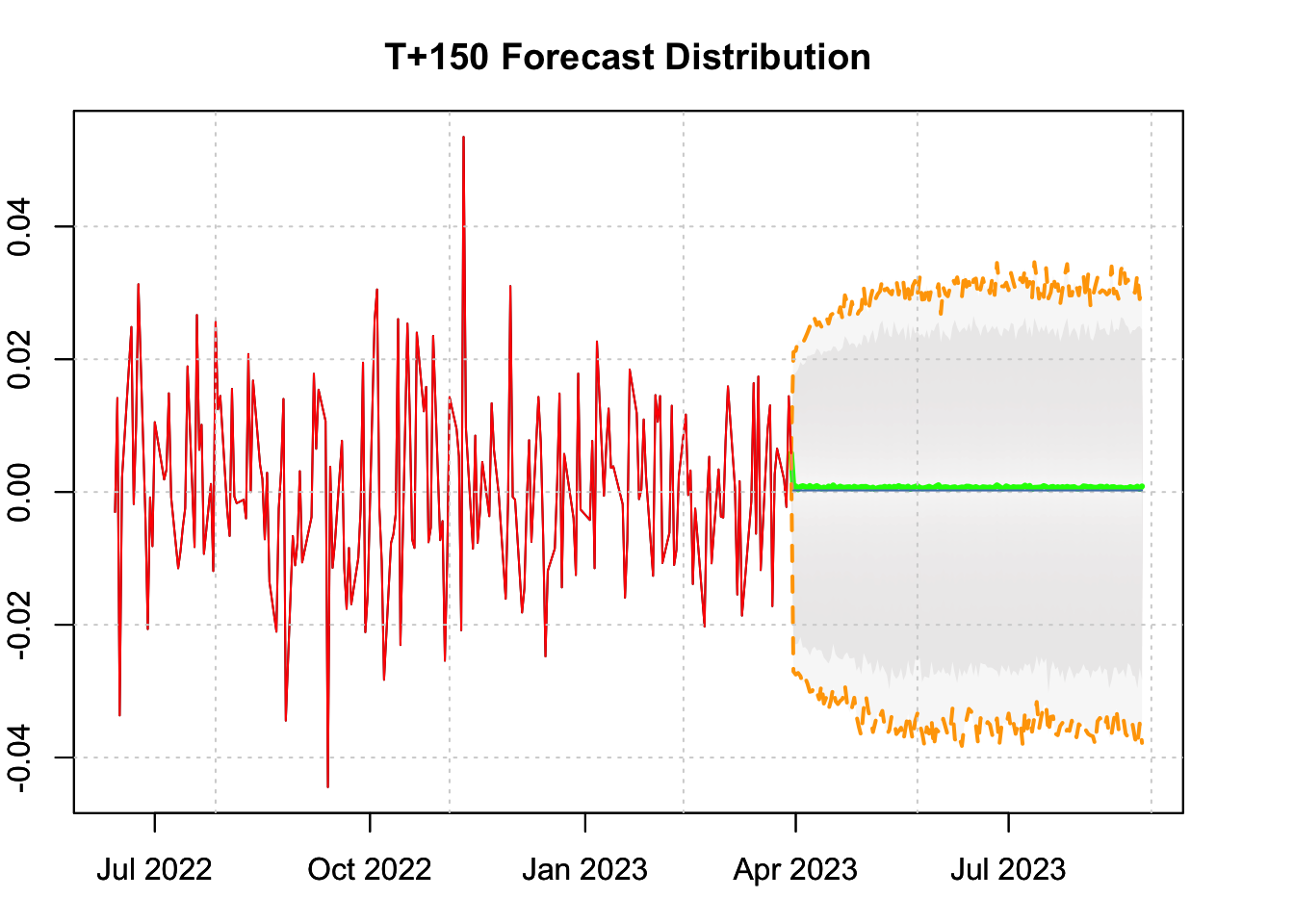
Finally, we can just plot the predicted object which contains the simulated predictive density of the model.

Code
par(mar = c(3,2,3,3))
plot(p, n_original = 200, interval_quantile = c(0.01, 0.99), median_color = 'green', gradient_color = 'snow3', interval_color = "orange", main = "T+150 Forecast Distribution")
lines(index(p$mean), as.numeric(p$mean), col = 'steelblue')

3.4 Backtesting

The tsbacktest method allows the generation of rolling forecasts using an expanding window and returns the values needed to describe the forecast conditional density including the mean, sigma, skew, shape and lambda values, which may be of particular interest for evaluating value at risk or other distributional measures.

The backtest method has 2 key arguments, the forecast horizon (h) and the number of period before a model is re-estimated to generate a fresh set of parameters from which to forecast. In the case of rolling forecasts, the data is filtered (using the tsfilter method) every period in order to update the last state from which new forecasts of length h are generated. Forecasts are uniquely defined by their horizon and and forecast date.

The tsbacktest method across all packages in the tsmodels framework allows the use of parallel processing via the future package.

Code
# create a mew specification
spec <- garch_modelspec(r, model = "egarch", constant = TRUE, distribution = "jsu")
# set up resources
library(future)
plan("future::multisession", workers = 10)
b <- tsbacktest(spec, start = 7000, h = 10, estimate_every = 30, rolling = TRUE, trace = FALSE)
# return to sequential
plan("future::sequential")

The main component of the returned list is a table with the following headings:

Code
print(b$table, topn = 2, trunc.cols = T)
##       estimation_date convergence filter_date horizon
##                <Date>       <int>      <Date>   <int>
##    1:      2020-11-13           1  2020-11-13       1
##    2:      2020-11-13           1  2020-11-13       2
##   ---                                                
## 5914:      2023-02-22           1  2023-03-28       2
## 5915:      2023-02-22           1  2023-03-29       1
## 8 variables not shown: [size <int>, forecast_date <Date>, mu <num>, sigma <num>, skew <num>, shape <num>, lambda <num>, actual <num>]

The estimation_date shows the date on which the model was estimated from which the parameters were used for the forecast. It also outputs a convergence code which returns 1 if both the Kuhn-Karush-Tucker conditions (gradient and positive definite Hessian) were satisfied8, else 0 which may mean that one or both conditions were not satisfied. The filter date is \(t_0\) date on which the forecast was made, with horizon denoting the n-ahead period forecast, size the expanding window size used for estimating the model and foreacast_date the date the forecast corresponds to. The remaining column headings are the forecasts of the conditional mean (mu) and volatility (sigma) and any additional distributional parameters (which are fixed based on the estimated model). Note that even if the model has no additional distributional parameters, the defaults will still be printed since the (d,p,q,r) methods from the tsdistribution package can take all this information, given some distribution, and will take care of which distribution needs what. Finally, the actual column is the realized value of y for each forecast_date.

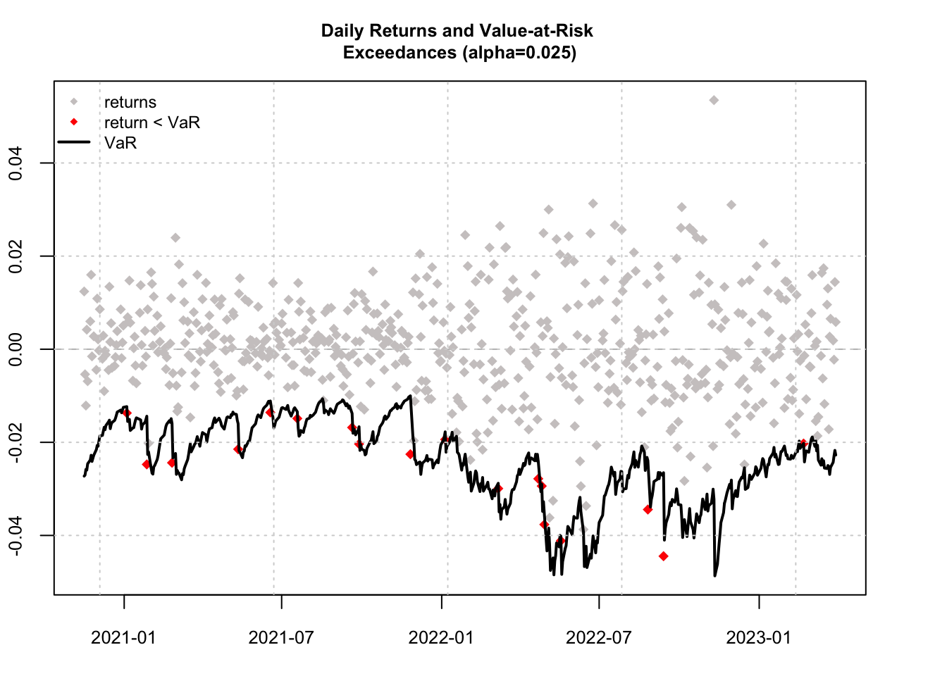
An interesting way to visualize the 1-step ahead forecasts is by looking at the value at risk exceedances plot:

Code
library(tsdistributions)
h1 <- b$table[horizon == 1, .(filter_date, forecast_date, mu, sigma, skew, shape, lambda, actual)]
h1[,VaR := qdist(b$distribution, p = 0.025, mu = mu, sigma = sigma, skew = skew, shape = shape, lambda = lambda)]
main_title <-  paste("Daily Returns and Value-at-Risk \nExceedances (alpha=0.025)",sep = "")
par(mar = c(3,2,3,3))
plot(h1$forecast_date, h1$actual, type = "n", main = title, ylim =
         c(min(min(h1$actual), min(h1$VaR)),
           max(max(h1$actual), max(h1$VaR))),
     ann = FALSE, cex.lab = 0.9, cex.axis = 0.8)
title(main_title, cex.main = 0.8)
abline(h = 0, col = "grey", lty = 2)
points(h1$forecast_date, h1$actual, pch = 18, col = "snow3")
sel <- which(h1$actual < h1$VaR)
points(h1$forecast_date[sel],h1$actual[sel], pch = 18, col = "red")
lines(h1$forecast_date, h1$VaR, lwd = 2, col = "black")
legend("topleft", max(h1$actual), c("returns","return < VaR","VaR"),
       col = c("snow3", "red","black"), cex = 0.75,
       pch = c(18,18,-1), lty = c(0,0,1), lwd = c(0,0,2), bty = "n")
grid()

3.5 Benchmark

The package has a built-in function which generates a table for the benchmark of Fiorentini, Calzolari, and Panattoni (1996), showing the log relative error between the values from tsgarch and the benchmark values, and defined as:

\[ \textrm{LRE} = -\log_{10}\left(\frac{\left|x - b\right|}{\left|b\right|}\right) \] where \(x\) is the estimated value and \(b\) the benchmark value.

Code
benchmark <- benchmark_fcp()
as_flextable(benchmark)

Estimate

Std Error (H)

Std Error (OPG)

Std Error (QML)

tsgarch

FCP

tsgarch

FCP

tsgarch

FCP

tsgarch

FCP

μ\mu

-0.0062

-0.0062

0.0085

0.0085

0.0084

0.0084

0.0092

0.0092

6.1211

6.9780

6.4183

6.3680

ω\omega

0.0108

0.0108

0.0029

0.0029

0.0013

0.0013

0.0065

0.0065

5.0396

6.1361

5.4328

6.2615

α1\alpha_1

0.1531

0.1531

0.0265

0.0265

0.0140

0.0140

0.0535

0.0535

6.3890

5.9351

5.1806

7.4256

β1\beta_1

0.8060

0.8060

0.0336

0.0336

0.0166

0.0166

0.0725

0.0725

6.3835

6.5139

6.7485

6.1570

Notes to table: values in italic are the log relative errors (LRE). The FCP benchmark is from the paper by Fiorentini, G., G. Calzolari and L. Panattoni, Analytic Derivatives and the Computation of GARCH Estimates, Journal of Applied Econometrics 11 (1996), 399--417.

4 Conclusion

The package is still in active development. Additional models may be added, porting some of the remaining rugarch models, but the focus is likely to be on models for high frequency data and porting the multivariate models from rmgarch.

A separate package called tstests includes a number of tests which were previously part of rugarch and is already on CRAN.

5 Appendix

5.1 Methods and Classes

(...)

type

input

output

tsgarch                   

¦--garch_modelspec       

function

xts

tsgarch.spec

¦   ¦--simulate          

method

tsgarch.spec

tsgarch.simulate

¦   ¦--tsfilter          

method

tsgarch.spec

tsgarch.estimate

¦   ¦--omega             

method

tsgarch.spec

numeric

¦   °--tsbacktest        

method

tsgarch.spec

list

¦--estimate              

method

tsgarch.spec

tsgarch.estimate

¦   ¦--summary           

method

tsgarch.estimate

summary.tsgarch

¦   ¦   ¦--print         

method

summary.tsgarch

print

¦   ¦   °--as_flextable  

method

summary.tsgarch

flextable

¦   ¦--tidy              

method

tsgarch.estimate

tibble

¦   ¦--glance            

method

tsgarch.estimate

tibble

¦   ¦--omega             

method

tsgarch.estimate

numeric

¦   ¦--sigma             

method

tsgarch.estimate

numeric

¦   ¦--plot              

method

tsgarch.estimate

plot

¦   ¦--coef              

method

tsgarch.estimate

numeric

¦   ¦--logLik            

method

tsgarch.estimate

logLik

¦   ¦--fitted            

method

tsgarch.estimate

xts

¦   ¦--residuals         

method

tsgarch.estimate

xts

¦   ¦--tsequation        

method

tsgarch.estimate

list

¦   ¦--AIC               

method

tsgarch.estimate

numeric

¦   ¦--BIC               

method

tsgarch.estimate

numeric

¦   ¦--persistence       

method

tsgarch.estimate

numeric

¦   ¦--confint           

method

tsgarch.estimate

matrix

¦   ¦--vcov              

method

tsgarch.estimate

matrix

¦   ¦--bread             

method

tsgarch.estimate

matrix

¦   ¦--estfun            

method

tsgarch.estimate

matrix

¦   ¦--predict           

method

tsgarch.estimate

tsmodel.predict

¦   ¦   ¦--plot          

method

tsmodel.predict

plot

¦   ¦   °--pit           

method

tsgarch.predict

xts

¦   ¦--simulate          

method

tsgarch.estimate

tsmodel.simulate

¦   ¦--tsfilter          

method

tsgarch.estimate

tsmodel.estimate

¦   ¦--unconditional     

method

tsgarch.estimate

numeric

¦   ¦--nobs              

method

tsgarch.estimate

numeric

¦   °--pit               

method

tsgarch.estimate

xts

¦--halflife              

method

numeric

numeric

¦--newsimpact            

function

numeric

tsgarch.newsimpact

¦   °--plot              

method

tsgarch.newsimpact

plot

¦--arma_coefficients     

function

tsgarch.estimate

list

¦--arma_inverse_roots    

function

tsgarch.estimate

list

¦--arma_irf              

function

tsgarch.estimate

list

°--arma_near_cancellation

function

list

data.table

6 References

Barndorff-Nielsen, Ole, and Geert Schou, 1973, On the parametrization of autoregressive models by partial autocorrelations, Journal of Multivariate Analysis 3, 408–419.
Bollerslev, T., 1986, Generalized autoregressive conditional heteroskedasticity, Journal of Econometrics 31, 307–327.
Caporin, Massimiliano, and Michele Costola, 2019, Asymmetry and leverage in GARCH models: A news impact curve perspective, Applied Economics 51, 3345–3364.
Charles, Amélie, and Olivier Darné, 2019, The accuracy of asymmetric GARCH model estimation, International Economics 157, 179–202.
Ding, Z., C. W. J. Granger, and R. F. Engle, 1993, A long memory property of stock market returns and a new model, Journal of Empirical Finance 1, 83–106.
Engle, R. F., 1982, Autoregressive conditional heteroscedasticity with estimates of the variance of united kingdom inflation, Econometrica 50(4), 987–1007.
Engle, R.F., and T. Bollerslev, 1986, Modelling the persistence of conditional variances, Econometric Reviews 5, 1–50.
Engle, Robert F, and Victor K Ng, 1993, Measuring and testing the impact of news on volatility, The Journal of Finance 48, 1749–1778.
Fiorentini, Gabriele, Giorgio Calzolari, and Lorenzo Panattoni, 1996, Analytic derivatives and the computation of GARCH estimates, Journal of Applied Econometrics 11, 399–417.
Francq, Christian, Lajos Horvath, and Jean-Michel Zakoian, 2011, Merits and drawbacks of variance targeting in GARCH models, Journal of Financial Econometrics 9, 619–656.
Glosten, L.R., R. Jagannathan, and D.E. Runkle, 1993, On the relation between the expected value and the volatility of the nominal excess return on stocks, Journal of Finance 48(5), 1779–1801.
Hansen, Bruce E, 1994, Autoregressive conditional density estimation, International Economic Review, 705–730.
He, Changli, Timo Terasvirta, and Hans Malmsten, 2002, Moment structure of a family of first-order exponential GARCH models, Econometric Theory 18, 868–885.
Hentschel, L., 1995, All in the family nesting symmetric and asymmetric GARCH models, Journal of Financial Economics 39, 71–104.
Hill, Chelsey, and BD McCullough, 2019, On the accuracy of garch estimation in r packages, Econometric Research in Finance 4, 133–156.
Jones, Richard H, 1980, Maximum likelihood fitting of ARMA models to time series with missing observations, Technometrics 22, 389–395.
Laurent, Sebastien, 2004, Analytical derivates of the APARCH model, Computational Economics 24, 51–57.
Lee, G. J., and R. F. Engle, 1999, A permanent and transitory component model of stock return volatility, Cointegration causality and forecasting a festschrift in honor of clive WJ granger (Oxford University Press).
Nelson, Daniel B, 1990, Stationarity and persistence in the GARCH (1, 1) model, Econometric theory 6, 318–334.
Nelson, Daniel B, 1991, Conditional heteroskedasticity in asset returns: A new approach, Econometrica: Journal of the Econometric Society, 347–370.
Newey, Whitney K, and Kenneth D West, 1994, Automatic lag selection in covariance matrix estimation, The Review of Economic Studies 61, 631–653.
Pascual, L., J. Romo, and E. Ruiz, 2006, Bootstrap prediction for returns and volatilities in GARCH models, Computational Statistics & Data Analysis 50, 2293–2312.
Rao, Singiresu S, 2019, Engineering Optimization: Theory and Practice (John Wiley & Sons).
Taylor, S.J., 1986, Modelling Financial Time Series (Wiley).
Yang, Kyung-won, and Tai-yong Lee, 2010, Heuristic scaling method for efficient parameter estimation, Chemical Engineering Research and Design 88, 520–528.
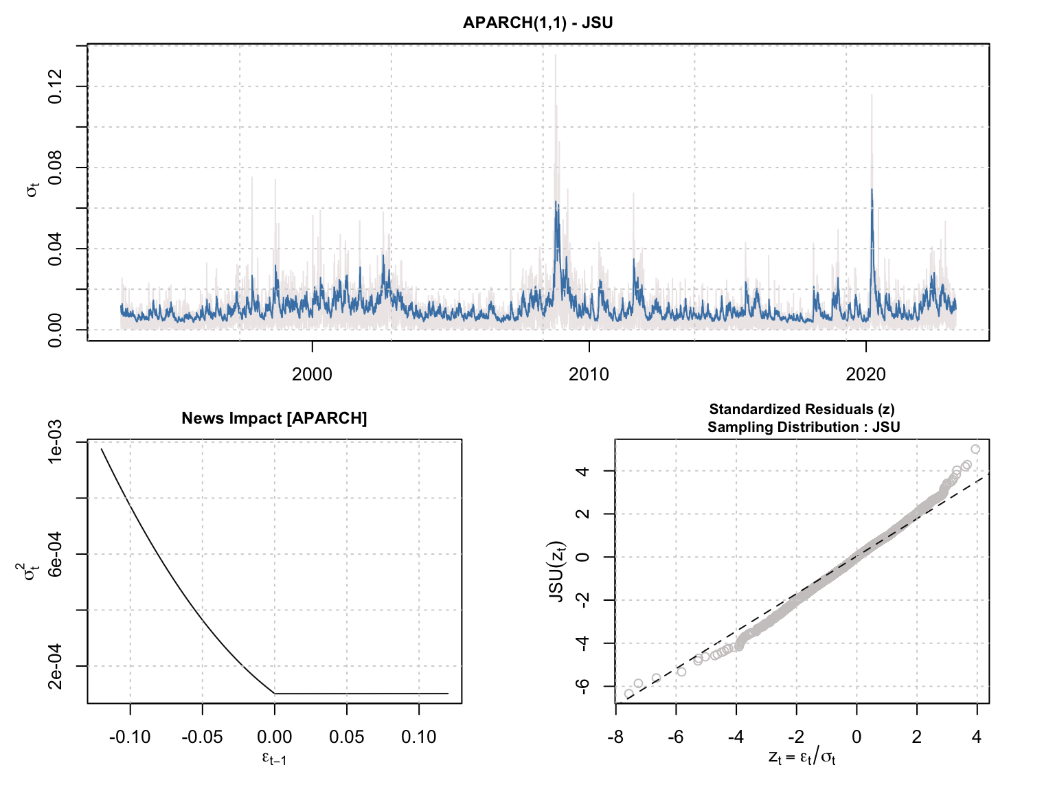
Back to top

Footnotes

  1. In the case when this assumption is relaxed, this will give rise to a non constant conditional distribution. See Hansen (1994).↩︎

  2. For some of the problems, the persistence has an easy closed form solution and therefore the Jacobian is hardcoded instead of making use of autodiff.↩︎

  3. Note that tsarma writes these coefficients \(\xi_k\); that symbol is already used in this package for the variance equation regressors (see Section Section 2.5), hence \(\tau_k\) here.↩︎

  4. If using a multiplicative intercept choice, then \(\bar\sigma^2 = \frac{\exp\left(\omega + \sum_{k=1}^n\xi_k\bar\chi_k\right)}{1 - P}\).↩︎

  5. Though many times it is also possible that this is the result of omitted structural breaks↩︎

  6. for details see the tsdistributions package.↩︎

  7. Some implementations in other software packages allow for more flexibility, allowing regressors to enter into both components.↩︎

  8. This is based on the kktchk function from the optimx package.↩︎