| Step | Specification Type | Operation | Resulting Object/Class |
|---|---|---|---|
| Manual Specification (auto = FALSE) | |||
| Model Specification | Manual (auto = FALSE) | issm_modelspec(auto = FALSE) | tsissm.spec |
| Estimation | Manual (auto = FALSE) | estimate() | tsissm.estimate |
| Backtesting | Manual (auto = FALSE) | tsbacktest() | Backtest output |
| Automatic Specification (top_n = 1) | |||
| Model Specification | Auto (top_n = 1) | issm_modelspec(auto = TRUE, top_n = 1) | tsissm.autospec |
| Estimation | Auto (top_n = 1) | estimate() | tsissm.estimate |
| Diagnostics & Summary | Auto (top_n = 1) | summary(), AIC(), BIC(), estfun(), bread(), residuals(), fitted(), tsdecompose(), tsmetrics(), vcov(), sigma(), logLik(), coef(), hresiduals(), tsequation(), tsdiagnose(), plot(), tsmoments(), tsprofile() |
Diagnostic outputs |
| Filtering | Auto (top_n = 1) | tsfilter() | Updated tsissm.estimate |
| Prediction & Simulation | Auto (top_n = 1) | predict() & simulate() | tsissm.predict and tsissm.simulate |
| Prediction Diagnostics | Auto (top_n = 1) | tsmetrics(), plot(), tsdecompose() | Prediction diagnostic outputs |
| Automatic Specification (top_n > 1) | |||
| Model Specification | Auto (top_n > 1) | issm_modelspec(auto = TRUE, top_n = 2) | tsissm.autospec |
| Estimation | Auto (top_n > 1) | estimate() | tsissm.selection |
| Filtering | Auto (top_n > 1) | tsfilter() | Updated tsissm.selection |
| Prediction & Simulation | Auto (top_n > 1) | predict() & simulate() | tsissm.selection_predict and tsissm.selection_simulate |
| Backtesting | Auto (top_n > 1) | tsbacktest() | Backtest output |
| Selection Diagnostics | Auto (top_n > 1) | AIC(), BIC(), logLik(), tsensemble() | Diagnostic and ensemble outputs |
1 Introduction
The tsissm package implements the linear innovations state space model described by De Livera, Hyndman, and Snyder (2011)1 and incorporating trigonometric seasonality as used in the tbats function from the forecast package of Hyndman et al. (2024). However, tsissm differs significantly in both implementation and features. Key enhancements include:
Automatic differentiation and robust inference:
Estimation leverages automatic differentiation (autodiff), with multiple sandwich estimators available for standard error calculation. System forecastability and ARMA constraints are handled exactly via the nloptr solver using autodiff-based Jacobians.Flexible error distributions:
In addition to Gaussian errors, the model supports heavy-tailed and skewed alternatives, including the Student’s \(t\) distribution and the Johnson’s SU distribution.Heteroscedasticity modeling:
Conditional heteroscedasticity is supported via a GARCH specification on the innovation variance.Automatic model selection and ensembling:
Users may select the best model based on an information criterion (e.g., AIC or BIC) or retain the top \(N\) models for ensembling. This feature is also available in thebacktestmethod, providing a more robust approach to evaluation and forecasting.Simulated predictive distributions:
Thepredictmethod always returns a simulated forecast distribution, alongside the analytic mean, allowing for richer uncertainty quantification.Handling of missing data:
Missing values in the response variable are permitted and automatically handled via the state space formulation.Support for external regressors:
Regressors are supported in both the mean equation.2
2 Model Formulation
Given an initial state vector of unobserved components (such as level, slope, and seasonality), the proposed model evolves the states over time using a linear transition equation, incorporating the effect of the most recent observation error. At each time step, the observed (Box-Cox transformed) value is modeled as a linear combination of the previous state, lagged external regressors, and a normally3 distributed random error. This structure allows the model to capture complex patterns in the data—such as trends, seasonal cycles, and the influence of exogenous variables—while dynamically updating its internal state based on new information.
Consider the following Single Error Model (SEM) with trigonometric seasonality:
\[ \begin{aligned} y_t^{(\lambda)} &= {\bf{w'}}{{\bf{x}}_{t - 1}} + \bf{c'}\bf{u}_{t - 1} + {\varepsilon _t}, \quad \varepsilon_t\sim N\left(0,\sigma^2\right),\\ {{\bf{x}}_t} &= {\bf{F}}{{\bf{x}}_{t - 1}} + {\bf{g}}{\varepsilon _t}, \end{aligned} \tag{1}\]
where \(\lambda\) represents the Box Cox parameter, \(\bf{w}\) the observation coefficient vector, \(\bf{x}_t\) the unobserved state vector, and \(\bf{c}\) a vector of coefficients on the external regressor set \(\bf{u}\).4
Define the state vector5 as:
\[ \bf{x}_t = {\left( {{l_t},{b_t},s_t^{(1)},\dots,s_t^{(T)},{d_t},{d_{t - 1}},\dots,{d_{t - p - 1}},{\varepsilon_t},{\varepsilon_{t - 1}},\dots,{\varepsilon _{t - q - 1}}} \right)^\prime }, \tag{2}\]
where \(\bf{s}_t^{(i)}\) is the row vector \(\left( {s_{1,t}^{(i)},s_{2,t}^{(i)},\dots,s_{{k_i},t}^{(i)},s_{1,t}^{*(i)},s_{2,t}^{*(i)},\dots,s_{{k_i},t}^{*(i)}} \right)\) for the trigonometric seasonality. Also define \(\bf{1}_r\) and \(\bf{0}_r\) as a vector of ones and zeros, respectively, of length \(r\), \(\bf{O}_{u,v}\) a \(u\times v\) matrix of zeros and \(\bf{I}_{u,v}\) a \(u\times v\) diagonal matrix of ones; let \(\mathbf{\gamma} = \left(\mathbf{\gamma}^{(1)},\dots,\mathbf{\gamma}^{(T)} \right)\) be a vector of seasonal parameters with \({\gamma ^{(i)}} = \left( {\gamma _1^{(i)}{{\bf{1}}_{{k_i}}},\gamma _2^{(i)}{{\bf{1}}_{{k_i}}}} \right)\) (with \(k\) harmonics); \(\theta = \left( {{\theta_1},{\theta_2},\dots,{\theta _p}} \right)\) and \(\psi = \left( {{\psi _1},{\psi _2},\dots,{\psi_q}} \right)\) as the vector of AR(p) and MA(q) parameters, respectively. The observation transition vector \({\bf{w}} = {\left( {1,\phi ,{\bf{a}},\theta ,\psi } \right)^\prime }\), where \({\bf{a}} = \left( {{{\bf{a}}^{(1)}},\dots,{{\bf{a}}^{(T)}}} \right)\) with \({{\bf{a}}^{(i)}} = \left( {{{\bf{1}}_{{k_i}}},{{\bf{0}}_{{k_i}}}} \right)\). The state error adjustment vector \({\bf{g}} = {\left( {\alpha ,\beta ,\gamma ,1,{{\bf{0}}_{p - 1}},1,{{\bf{0}}_{q - 1}}} \right)^\prime }\). Further, let \({\bf{B}} = \gamma '\theta\), \({\bf{C}} = \gamma '\psi\) and \({\bf{A}} = \oplus _{i = 1}^T{{\bf{A}}_i}\), with
\[ {{\bf{A}}_i} = \left[ {\begin{array}{*{20}{c}} {{{\bf{C}}^{(i)}}}&{{{\bf{S}}^{(i)}}}\\ { - {{\bf{S}}^{(i)}}}&{{{\bf{C}}^{(i)}}} \end{array}} \right], \tag{3}\]
and with \(\bf{C}^{(i)}\) and \(\bf{S}^{(i)}\) representing the \(k_i\times k_i\) diagonal matrices with elements \(cos(\lambda_j^{(i)})\) and \(sin(\lambda_j^{(i)})\)6 respectively.7
Finally, the state transition matrix \(\bf{F}\) is composed as follows:
\[ {\bf{F}} = \left[ {\begin{array}{*{20}{c}} 1&\phi &{{{\bf{0}}_\tau }}&{\alpha \theta }&{\alpha \psi }\\ 0&\phi &{{{\bf{0}}_\tau }}&{\beta \theta }&{\beta \psi }\\ {{{{\bf{0'}}}_\tau }}&{{{{\bf{0'}}}_\tau }}&{\bf{A}}&{\bf{B}}&{\bf{C}}\\ 0&0&{{{\bf{0}}_\tau }}&\theta &\psi \\ {{{{\bf{0'}}}_{p - 1}}}&{{{{\bf{0'}}}_{p - 1}}}&{{{\bf{O}}_{p - 1,\tau }}}&{{{\bf{I}}_{p - 1,p}}}&{{{\bf{O}}_{p - 1,q}}}\\ 0&0&{{{\bf{0}}_\tau }}&{{{\bf{0}}_p}}&{{{\bf{0}}_q}}\\ {{{{\bf{0'}}}_{q - 1}}}&{{{{\bf{0'}}}_{q - 1}}}&{{{\bf{O}}_{q - 1,\tau }}}&{{{\bf{O}}_{q - 1,p}}}&{{{\bf{I}}_{q - 1,q}}} \end{array}} \right] \tag{4}\]
where \(\tau = 2\sum\limits_{i = 1}^T {{k_i}}\). The model has the feature of allowing for multiple seasonal trigonometric components.
3 State Initialization
A key innovation of the De Livera, Hyndman, and Snyder (2011) paper is in providing the exact initialization of the non-stationary component’s seed states, the exponential smoothing analogue of the De Jong (1991) method for augmenting the Kalman filter to handle seed states with infinite variances. The proof, based on De Livera, Hyndman, and Snyder (2011) and expanded here is as follows, let:
\[ {\bf{D}} = {\bf{F}} - {\bf{gw'}}. \tag{5}\]
We eliminate \(\varepsilon_t\) in Equation 1 to give:
\[ {\bf{x}}_t = \bf{D}{\bf{x}_{t - 1}} + \bf{g}{y_t}. \tag{6}\]
Next, we proceed by backsolving the equation for the error, given a given value of \(\lambda\):8
\[ \begin{array}{l} {\varepsilon_t} = {y_t} - {\bf{w}}{{{\bf{\hat x}}}_{t - 1}},\\ {\varepsilon_t} = {y_t} - {\bf{w'}}\left({{\bf{D}}{{{\bf{\hat x}}}_{t - 2}} + {\bf{g}}{y_{t - 1}}}\right). \end{array} \tag{7}\]
Starting with \(t = 4\) and working backwards:
\[ \begin{array}{rl} {\varepsilon_4} &= {y_4} - {\bf{w'}}\left({\bf{D}}{{{\bf{\hat x}}}_2} + {\bf{g}}{y_3} \right)\\ &= {y_4}-{\bf{w'}}\left({{\bf{D}}\left({\bf{D}}{{{\bf{\hat x}}}_1} + {\bf{g}}{y_2} \right) + {\bf{g}}{y_3}} \right)\\ &= {y_4}-{\bf{w'}}\left({{\bf{D}}\left({{\bf{D}}\left( {{\bf{D}}{{{\bf{\hat x}}}_0} + {\bf{g}}{y_1}} \right) + {\bf{g}}{y_2}} \right) + {\bf{g}}{y_3}} \right)\\ &= {y_4}-{\bf{w'}}\left({{\bf{D}}\left({{\bf{D}}^2}{{\bf{x}}_0} + {\bf{Dg}}{y_1} + {\bf{g}}{y_2}\right) + {\bf{g}}{y_3}} \right)\\ &= {y_4}-{\bf{w'}}\left({{\bf{D}}^3}{{\bf{x}}_0} + {{\bf{D}}^2}{\bf{g}}{y_1} + {\bf{Dg}}{y_2} + {\bf{g}}{y_3}\right)\\ &= {y_4}-{\bf{w'}}\sum\limits_{j = 1}^3 {{\bf{D}}^{j - 1}}{\bf{g}}{y_{4 - j}} - {\bf{w'}}{{\bf{D}}^3}{{\bf{x}}_0}\\ \end{array} \tag{8}\]
and generalizing to \(\varepsilon_t\):
\[ \begin{array}{rl} {\varepsilon_t} &= {y_t} - {\bf{w'}}\left( {\sum\limits_{j = 1}^{t - 1} {{{\bf{D}}^{j - 1}}{\bf{g}}{y_{t - j}}} } \right) - {\bf{w'}}{{\bf{D}}^{t - 1}}{{\bf{x}}_0}\\ &= {y_t} - {\bf{w'}}{{{\bf{\tilde x}}}_{t - 1}} - {{{\bf{w'}}}_{t - 1}}{{\bf{x}}_0}\\ &= {{\tilde y}_t} - {{{\bf{w'}}}_{t - 1}}{{\bf{x}}_0}, \end{array} \tag{9}\]
where \({{\tilde y}_t} = {y_t} - {\bf{w'}}{{{\bf{\tilde x}}}_{t - 1}}\), \({{{\bf{\tilde x}}}_t} = {\bf{D}}{{{\bf{\tilde x}}}_{t - 1}} + {\bf{g}}{y_t}\), \({{{\bf{w'}}}_t} = {\bf{D}}{{{\bf{w'}}}_{t - 1}}\), \({{{\bf{\tilde x}}}_0} = 0\) and \({{{\bf{w'}}}_0} = {\bf{w'}}\), so that \(\bf{x}_0\) are the coefficients from the regression of \(\bf{w}\) on \(\boldsymbol{\varepsilon}\). The way this is implemented, is to calculate the seed states based on the initial parameter vector and \(\lambda\) parameter and then use those same seed states without re-calculating during the optimization. However, when \(\lambda\) is also part of the parameter estimation set, we have chosen instead to re-calculate the seed state during the optimization as part of the autodiff tape. This differs from the approach adopted in the forecast package of Hyndman et al. (2024) which simply re-transforms the initial seed states based on the value of \(\lambda\) during estimation.
4 Constraints
A number of constraints are implemented during estimation, including a system forecastability constraint and a constraint on the ARMA parameters when present.
4.1 System Forecastability Constraint
The forecastability constraint necessitates that the characteristic roots of the matrix \(D\) (see Equation 5) lie within the unit circle, which means that the maximum of the modulus of the eigenvalues of D are less than 1. In the forecast package this constraint is directly checked and returns Inf when the condition is violated which is a type of infinite penalty method. It is known that this type of approach can lead to numerical instabilities and discontinuities as well as difficulties in convergence, though it often “works” in practice to some degree. Instead, in the tsissm package, we model the constraint using RTMB9 to obtain the autodiff based Jacobian of the constraint and pass the output to the nloptr solver using the eval_g_ineq and eval_jac_g_ineq arguments. Specifically, in order to avoid the use of the non-differentiable \(max\) operator, we impose that the modulus of all the eigenvalues is less than 1 and the Jacobian is then a \(C \times N\) matrix where \(C\) are the constraints and \(N\) the number of parameters.10
4.2 ARMA Constraint
It is typical to check for stationarity in the AR component and invertibility in the MA component when those are present, by solving for the characteristic roots of the system polynomials. In R, one way to solve for this is to use the polyroot function such that Mod(polyroot(c(1, -ar))) and Mod(polyroot(c(1, ma))) are greater than 1. In the forecast package this is how they are checked and an infinite penalty applied, similar to the system forecastability constraint. As in our previous approach, we instead code this up to make use of automatic differentiation in order to obtain a reasonable set of constraints and their Jacobians.
Consider an autoregressive (AR) model specified by the polynomial
\[ 1 - a_1 z - a_2 z^2 - \cdots - a_n z^n = 0. \]
The stationarity condition requires that the roots \(z\) of this polynomial satisfy \(|z| > 1.\)
That is, the roots must lie outside the unit circle.
Multiply the equation by \(-1\) to obtain:
\[ -1 + a_1 z + a_2 z^2 + \cdots + a_n z^n = 0. \]
Rearrange this as:
\[ a_n z^n + a_{n-1} z^{n-1} + \cdots + a_1 z - 1 = 0. \]
Dividing through by \(a_n\) (assuming \(a_n \neq 0\)) yields the monic polynomial:
\[ z^n + \frac{a_{n-1}}{a_n} z^{n-1} + \cdots + \frac{a_1}{a_n} z - \frac{1}{a_n} = 0. \]
For a monic polynomial
\[ z^n + c_{n-1} z^{n-1} + \cdots + c_1 z + c_0 = 0, \]
the standard companion matrix is defined as:
\[ C = \begin{pmatrix} - c_{n-1} & - c_{n-2} & \cdots & - c_1 & - c_0 \\ 1 & 0 & \cdots & 0 & 0 \\ 0 & 1 & \cdots & 0 & 0 \\ \vdots & \vdots & \ddots & \vdots & \vdots \\ 0 & 0 & \cdots & 1 & 0 \end{pmatrix}. \]
In our case, by comparing coefficients, we have:
\[ c_{n-1} = \frac{a_{n-1}}{a_n},\quad c_{n-2} = \frac{a_{n-2}}{a_n},\quad \dots,\quad c_1 = \frac{a_1}{a_n},\quad c_0 = -\frac{1}{a_n}. \]
Thus, the companion matrix becomes:
\[ C = \begin{pmatrix} -\dfrac{a_{n-1}}{a_n} & -\dfrac{a_{n-2}}{a_n} & \cdots & -\dfrac{a_1}{a_n} & \dfrac{1}{a_n} \\ 1 & 0 & \cdots & 0 & 0 \\ 0 & 1 & \cdots & 0 & 0 \\ \vdots & \vdots & \ddots & \vdots & \vdots \\ 0 & 0 & \cdots & 1 & 0 \end{pmatrix}. \]
Since the eigenvalues of the companion matrix ( C ) are precisely the roots ( z ) of the polynomial
\[ 1 - a_1 z - a_2 z^2 - \cdots - a_n z^n = 0, \]
the stationarity condition \(|z| > 1\) can be reformulated in terms of the companion matrix as
\[ |\lambda_i(C)| > 1 \quad \text{for } i = 1, \dots, n. \]
That is, the moduli of the eigenvalues of the companion matrix must be greater than 1. A detailed exposition can be found in Lütkepohl (2005) (see Chapter 3).
A similar constraint is imposed in the presence of an MA component, by flipping the sign of the coefficients. It should be noted that these constraints are only applied when the order of either the AR or MA components is greater than 1, else the normal parameter bounds ({-1, 1}) are sufficient.
5 Estimation
The estimation is carried out by minimizing the negative of the log-likelihood, subject to various constraints discussed in Section 4, and parameter bounds. The log-likelihood (to be maximized), jointly with the Box-Cox transformation (parameter \(\lambda\)) is derived as follows:
\[ \begin{aligned} p(y_t \mid x_0, \vartheta, \sigma^2) &= p\left(y_t^{(\lambda)} \mid x_0, \vartheta, \sigma^2\right) \,\det\!\left(\frac{\partial y_t^{(\lambda)}}{\partial y}\right)\\ &= p\left(y_t^{(\lambda)} \mid x_0, \vartheta, \sigma^2\right) \,\prod_{t=1}^n y_t^{\lambda - 1}\\ &= \ln p\left(y_t^{(\lambda)} \mid x_0, \vartheta, \sigma^2\right) \;+\; (\lambda - 1) \sum_{t=1}^n \ln y_t. \end{aligned} \tag{10}\]
where \(p(\cdot)\) represents the probability density function, given the initial state observations \(x_0\), the parameter vector \(\theta\) and the variance \(\sigma^2\).
The Box-Cox transformation, represented by parameter \(\lambda\) is a power transformation applied to the dependent variable to stabilize its variance and to make its distribution closer to normal. This adjustment often leads to improved model estimation and inference. Since we are jointly estimating lambda, it is necessary to adjust the likelihood by the Jacobian of the transformation, which in the likelihood expression appears as the determinant term
\[ \det\!\left(\frac{\partial y_t^{(\lambda)}}{\partial y}\right), \]
which is equivalently expressed as
\[ \prod_{t=1}^n y_t^{\lambda - 1}. \]
This term scales the probability density correctly back to the original data scale, ensuring that the transformation is properly accounted for during estimation. Including the parameter \((\lambda)\) in the estimation process allows the model to choose the optimal transformation that best normalizes the data and stabilizes its variance.
Beyond the Gaussian distribution, the package also implements the Student’s t and Johnson’s SU, details of which can be found in the tsdistributions package. Additionally, the variance can follow GARCH dynamics such that:
\[ \sigma^2_t = \hat\sigma^2 \left(1 - P\right) + \sum\limits_{j=1}^{q} \alpha_j \varepsilon_{t-j}^2 + \sum\limits_{j=1}^{p} \beta_j \sigma_{t-j}^2 \tag{11}\]
where we impose a variance targeting intercept instead of estimating \(\omega\), with \(P\) being the persistence and \(\hat\sigma^2\) the unconditional variance. Initialization of the recursion can either use the full information set or a subsample (for more details see the online documentation of tsgarch).
The optimization is undertaken using the nloptr solver, making use of an autodiff based gradient for the parameters and autodiff based Jacobian for the constraints. The solver defaults to the use of the SQP variant, but other options are available via the issm_control function.
In order to calculate sandwich estimators11 for the standard errors, the scores (Jacobian) of the log-likelihood function need to be calculated. Due to the expense of this operation on large datasets, we have implemented asynchronous evaluation which requires the use of a parallel worker set up using a future plan. The user can also turn off the evaluation of scores, in which case the autodiff based Hessian is used for the calculation of the standard errors.
6 Prediction
The h-step ahead analytic mean and variance of the model, in the Box-Cox transformed space, are given by:
\[ E\left(y_{n+h|n}^{(\lambda)}\right) = \mu_{t+h} = \mathbf{w}' \mathbf{F}^{h-1}\mathbf{x}_n \]
\[ V\left(y_{n+h|n}^{(\lambda)}\right) = \sigma^2_{t+h} = \begin{cases} \hat\sigma^2, & \text{if } h = 1, \\[6pt] \hat\sigma^2 \left[1 + \displaystyle\sum_{j=1}^{h-1} c_j^2 \right], & \text{if } h \geq 2. \end{cases} \]
where \(c_j = w'F^{j-1}g\). For the mean, a reasonable approximation in back-transformed space, using a second-order Taylor expansion, is given by:
\[ y_{t+h} = \left\{ \begin{array}{ll} \exp(\mu_{t+h}) \left( 1 + \frac{\sigma^2_{t+h}}{2} \right), & \text{if } \lambda = 0, \\[8pt] (\lambda \mu_{t+h} + 1)^{\frac{1}{\lambda}} \left( 1 + \frac{\sigma^2_{t+h} (1-\lambda)}{2 (\lambda \mu_{t+h} + 1)^2} \right), & \text{if } \lambda \neq 0. \end{array} \right. \]
For the variance in the back transformed space, one should use the simulated distribution to approximate this as it was not possible to find a reasonable approximation, even using higher order Taylor expansions, which would be good enough, particularly with increasing h.
7 Automatic Selection and Ensembling
The forecast package of Hyndman et al. (2024) takes a smart, automated approach to identifying the best model from a set of candidate specifications—such as whether to include a slope, the number of harmonics, and the number of AR or MA terms.
In contrast, the tsissm package supports complete enumeration of all model configurations, including multiple seasonalities and multiple harmonics per seasonal frequency. It also allows testing for constant versus dynamic variance, though only one distributional assumption can be tested at a time. Users can return either the best model based on an information criterion (AIC or BIC), or the top \(N\) models ranked by the selected criterion. This flexibility enables model ensembling for filtering, prediction, and simulation.
The backtesting function (tsbacktest) supports this functionality directly, allowing automatic selection of the top \(N\) models. Three weighting schemes are available:
- User-supplied fixed weights.
- AIC-based weights:
Models are weighted by the Akaike Information Criterion, favoring those with lower AIC: \[ w_i = \frac{\exp(-0.5\, \Delta_i)}{\sum_{j} \exp(-0.5\, \Delta_j)}, \quad \text{where } \Delta_i = AIC_i - \min_j AIC_j. \] - BIC-based weights:
Similar to AIC-based weights, but using the Bayesian Information Criterion, which penalizes complexity more heavily.
The final ensemble prediction is computed as a weighted average: \[ \hat{y}_{\text{ensemble}} = \sum_{i} w_i\, \hat{y}_i, \] where \(\hat{y}_i\) are individual model predictions and \(w_i\) are the corresponding model weights. AIC-based weighting is typically preferred when models vary in complexity but are fit on the same dataset, whereas BIC-based weighting may be more appropriate for large sample sizes due to its stronger complexity penalty.
Beyond point forecasts, we also ensemble simulated forecasts, accounting for error dependencies across models. Rather than assuming independence, we explicitly model the dependence structure of model residuals using a Gaussian copula. This provides more accurate risk quantification, especially when the top \(N\) models are highly correlated.
First, the correlation of transformed residuals across retained models is computed using Kendall’s tau12. This is then converted into a correlation matrix \(\mathbf{R}\) suitable for a Gaussian copula:
\[ R_{k\ell} = \sin\left( \frac{\pi}{2} \tau^{(k,\ell)} \right). \]
From this, correlated quantile samples are drawn from a multivariate normal distribution and passed into the prediction function via the innov argument with innov_type = "q" (quantiles). These quantiles are then transformed back into residuals using each model’s error distribution, allowing for simulated forecasts with cross-model error dependence.
Formally, for each model \(k = 1, \dots, K\), simulation \(j\), and forecast horizon \(i\), we define the simulation equations:
\[ \begin{aligned} y_{j,i}^{(k)} &= \left(x_{i-1}^{(k)}\right)^\top w^{(k)} + \left(X_i^{(k)}\right)^\top \kappa^{(k)} + E_{j,i}^{(k)} \\ x_i^{(k)} &= F^{(k)} x_{i-1}^{(k)} + g^{(k)} E_{j,i}^{(k)} \end{aligned} \]
The simulated error term \(E_{j,i}^{(k)}\) is generated as:
\[ E_{j,i}^{(k)} = F_k^{-1} \left( \Phi\left(z_{j,i}^{(k)}\right) \right), \quad \text{where } \mathbf{z}_{j,i} \sim \mathcal{N}(\mathbf{0}, \mathbf{R}). \]
Here:
- \(\Phi(\cdot)\) is the standard normal cumulative distribution function (CDF),
- \(F_k^{-1}(\cdot)\) is the quantile function (inverse CDF) of the error distribution for model \(k\),
- \(z_{j,i}^{(k)}\) is the \(k\)-th element of the multivariate Gaussian sample,
- \(\mathbf{R}\) is the copula correlation matrix derived from Kendall’s tau between model residuals.
This approach preserves both marginal error distributions and cross-model error dependence in simulation-based forecasting.
8 Methods and Functions
Table 1 provides a summary of the methods and functions implemented in the package by input specification.
9 Demo: Missing Data
A recent blog post from Google Research introduced a compositional Bayesian neural network model and showcased it using the well-known monthly average \(CO_2\) concentrations from the Mauna Loa observatory. While the example is informative, the monthly series poses little challenge from a modeling perspective.
In contrast, this demo explores the daily Mauna Loa \(CO_2\) dataset, which introduces substantial complexity due to its irregular sampling — data is not available for every day of the year. This irregularity poses problems for seasonal modeling, as uneven time intervals distort lag relationships and degrade model inference.
We demonstrate how the tsissm package, which natively supports missing values, can be used to reframe irregular series onto a regular time grid with gaps — improving both seasonal modeling and forecast accuracy.
9.1 Data Investigation
We begin by visualizing the daily Mauna Loa \(CO_2\) series:
Code
data("maunaloa")
opar <- par(mfrow = c(1,1))
par(mar = c(2,2,2,2))
plot(zoo(maunaloa$co2, maunaloa$date), type = "l", xlab = "", ylab = "", main = "Mauna Loa Daily Average CO2")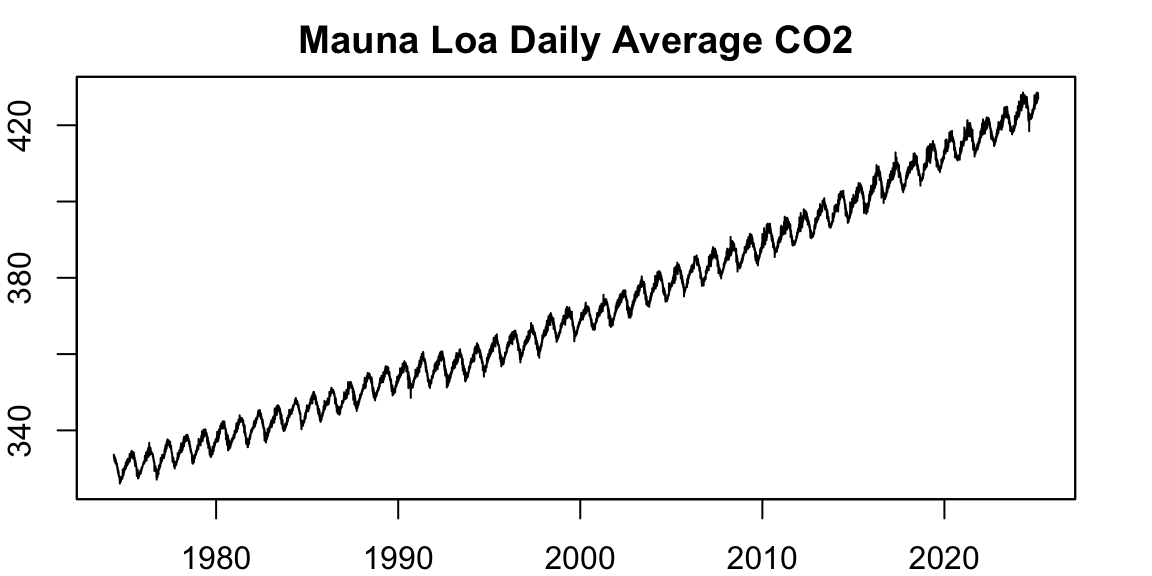
Code
par(opar)This dataset spans more than 20 years of daily averages. There is a clear seasonal pattern and a persistent upward trend. However, a closer look reveals that the number of observations per year is not constant:
Code
d <- data.table(date = maunaloa$date, value = maunaloa$co2)
d[, year := year(date)]
s <- d[,list(.N), by = "year"]
opar <- par(mfrow = c(1,1))
par(mar = c(2,2,2,2))
barplot(s$N, names.arg = s$year, main = "Observations/Year", col = "steelblue")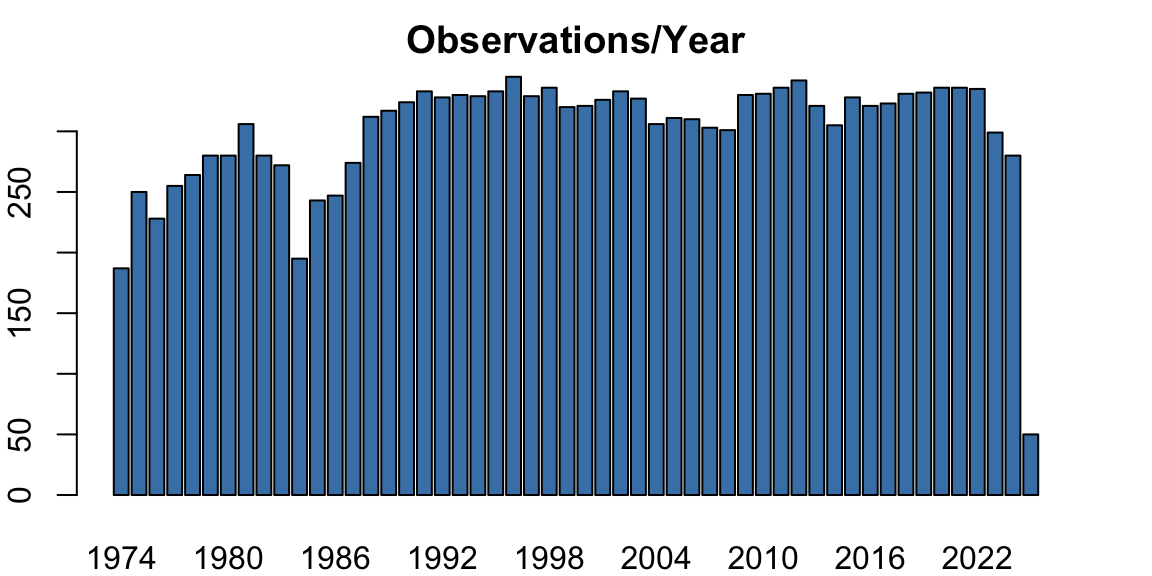
Code
par(opar)This inconsistency in daily coverage is the root of many issues when trying to fit seasonal models.
9.2 Naive Approach (Irregular Time Base)
A naive approach would be to directly model the series as-is, using a fixed seasonal frequency. For this example, we hold out the years 2024–2025 for evaluation:
Code
co2 <- xts(maunaloa$co2, maunaloa$date)
train <- co2["/2023"]
test <- co2["2024/"]
spec_naive <- issm_modelspec(train, slope = TRUE, seasonal = TRUE, seasonal_frequency = 320, seasonal_harmonics = 2)
# fixed slope
spec_naive$parmatrix[parameters == "beta", initial := 0]
spec_naive$parmatrix[parameters == "beta", lower := 0]
spec_naive$parmatrix[parameters == "beta", estimate := 0]
mod_naive <- estimate(spec_naive, scores = FALSE)
p_naive <- predict(mod_naive, h = length(test), nsim = 3000, forc_dates = index(test))
opar <- par(mfrow = c(1,1))
par(mar = c(2,2,2,2))
plot(p_naive, n_original = 600, gradient_color = "yellow", interval_color = "orange", main = "CO2 [Naive] Model Prediction", median_width = 1, xlab = "")
lines(index(test), as.numeric(test), col = 3)
legend("topleft", c("Median Forecast","Actual"), col = c(1,3), lty = 1, bty = "n")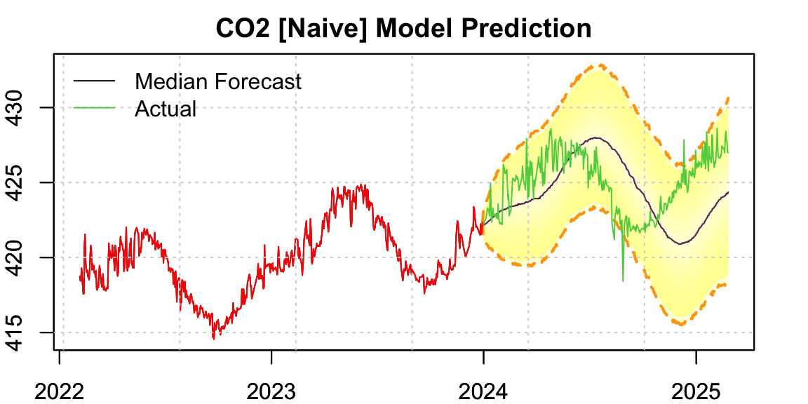
Code
par(opar)The resulting forecast exhibits a phase shift in the seasonal component. This is expected — irregular time spacing distorts seasonality, resulting in inaccurate timing of peaks and troughs.
9.3 Correct Approach (Regular Time Base with Missing Values)
A better solution is to recast the series on a regular daily time grid, filling in missing observations with NA. Since tsissm supports missing values in the response variable \(y_t\), this allows us to model the series in calendar time while preserving seasonal structure.
In tsissm, if y_t is missing, the innovation \(\varepsilon_t\) is set to zero — its expected value — effectively treating the model output as a one-step-ahead forecast. These missing values are ignored in the likelihood and handled correctly during state filtering.
Code
full_dates <- seq(index(co2)[1], tail(index(co2),1), by = "days")
co2_full <- xts(rep(as.numeric(NA), length(full_dates)), full_dates)
co2_full <- cbind(co2_full, co2, join = "left")
co2_full <- co2_full[,-1]
This new dataset now spans a regular daily grid. The percentage increase in data points (mostly NA) is: more data points which are all missing values.
9.4 Re-estimating with Regularized Calendar Time
Code
train_full <- co2_full["/2023"]
test_full <- co2_full["2024/"]
spec <- issm_modelspec(train_full, slope = TRUE, seasonal = TRUE, seasonal_frequency = 366, seasonal_harmonics = 5, distribution = "norm")
# fixed slope
spec$parmatrix[parameters == "beta", initial := 0]
spec$parmatrix[parameters == "beta", lower := 0]
spec$parmatrix[parameters == "beta", estimate := 0]
mod <- estimate(spec, scores = FALSE)
p <- predict(mod, h = length(test_full), nsim = 3000, forc_dates = index(test_full))
opar <- par(mfrow = c(1,1))
par(mar = c(2,2,2,2))
plot(p, n_original = 600, gradient_color = "yellow", interval_color = "orange", main = "CO2 [Correct] Model Prediction", median_width = 1, xlab = "")
lines(index(test_full), as.numeric(test_full), col = 3)
legend("topleft", c("Median Forecast","Actual"), col = c(1,3), lty = 1, bty = "n")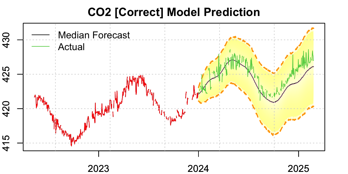
Code
par(opar)The forecast now clearly aligns better with the actual seasonal pattern — the phase error seen earlier has been corrected.
9.5 Evaluation
We compare forecast accuracy between the naive and corrected models using MAPE and CRPS. Only non-missing values are considered:
Code
use <- which(!is.na(as.numeric(test_full)))
tab <- data.frame(MAPE = c(mape(as.numeric(test), as.numeric(p_naive$analytic_mean)) * 100,
                           mape(as.numeric(test_full)[use], as.numeric(p$analytic_mean)[use]) * 100),
                  CRPS = c(crps(as.numeric(test), p_naive$distribution), crps(as.numeric(test_full)[use], p$distribution[,use])))
rownames(tab) <- c("Naive","Correct")
colnames(tab) <- c("MAPE (%)", "CRPS")
tab |> kable(digits = 2)| MAPE (%) | CRPS | |
|---|---|---|
| Naive | 0.55 | 1.57 |
| Correct | 0.26 | 0.77 |
The table shows a clear improvement in both metrics for the correctly specified model — particularly a halving of the MAPE.
9.6 Conclusion
Irregular sampling in time series — especially those with seasonal structure — can significantly impair model inference and forecasting. This demo demonstrated how naive models fitted on irregular time bases can introduce phase errors and bias. By recasting the series onto a regular grid with missing values, and leveraging tsissm’s built-in support for such data, we were able to restore seasonal fidelity and greatly improve forecast accuracy.
This approach is general and applicable to many real-world time series where regular sampling cannot be guaranteed.
10 Demo: Ensembling
The issm_modelspec() function is the primary entry point for modeling in the tsissm package. It defines a model specification with support for automatic selection across multiple configurations. In addition to selecting the single best model (e.g., by AIC), it can optionally return the top N ranked models, enabling downstream model ensembling for filtering, forecasting and simulation.
This demo showcases that functionality using U.S. Advanced Retail Sales data available in the package.
10.1 Advanced Retail Sales
This dataset represents the monthly, non-seasonally adjusted advance estimate of retail trade sales, based on a sub-sample of firms from the larger Monthly Retail Trade Survey.
As shown in the plot below, the series exhibits two prominent structural breaks: one around 2008 during the Global Financial Crisis, and another during the COVID-19 pandemic. To address this, we use the auto_regressors() function from the tsaux package, which detects and encodes three types of anomalies: additive outliers, temporary changes, and structural breaks (see this blog post for details).
Modeling such anomalies is important. When ignored, they are often absorbed by other components of the model, leading to biased coefficient estimates and inflated forecast variance.
Code
data("us_retail_sales")
opar <- par(mfrow = c(1,1))
y <- as.xts(us_retail_sales)
par(mar = c(2,2,2,2))
plot(as.zoo(y), ylab = "Sales (Mil's S)", xlab = "", main = "Advance Retail Sales")
grid()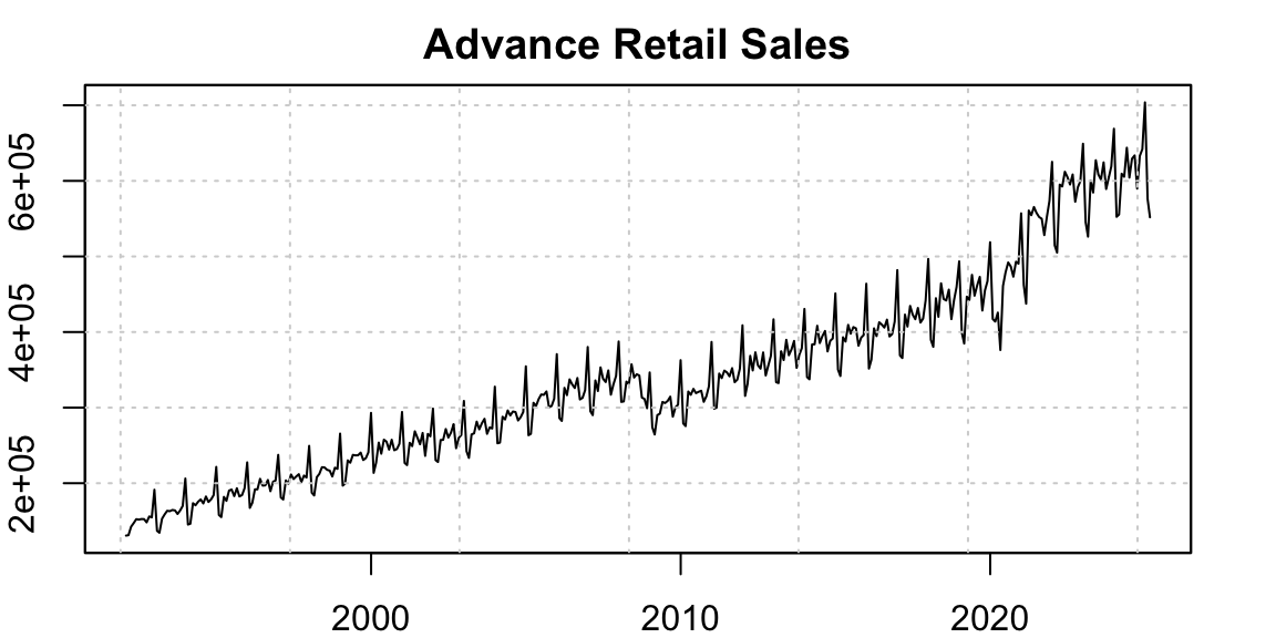
Code
par(opar)10.2 Model Selection
For this demonstration, we reserve the last 38 months of data for forecasting evaluation and select the top 4 models for ensembling.
Code
train <- y["/2021"]
test <- y["2022/"]
lambda_pre_estimate <- box_cox(lambda = NA)$transform(train) |> attr("lambda")
xreg <- auto_regressors(train, frequency = 12, lambda = lambda_pre_estimate, sampling = "months", h = 26, method = "sequential",
                        check.rank = TRUE, discard.cval = 3.5, maxit.iloop = 10, maxit.oloop = 10,
                        forc_dates = index(test))
spec <- issm_modelspec(train, auto = TRUE, slope = c(TRUE, FALSE), seasonal = TRUE,
                             seasonal_harmonics = list(c(3,4,5)), xreg = xreg$xreg[index(train), ],
                             seasonal_frequency = 12, ar = 0:2, ma = 0:2, lambda = lambda_pre_estimate, top_n = 4)
mod <- spec |> estimate()
We first inspect the top selected model:
Code
mod$models[[1]] |> summary() |> as_flextable()Estimate | Std. Error | t value | Pr(>|t|) | ||
|---|---|---|---|---|---|
| 0.3122 | 0.0388 | 8.0506 | 0.0000 | *** |
| 0.0000 | ||||
| -0.0035 | 0.0027 | -1.2960 | 0.1950 | |
| 0.0036 | 0.0015 | 2.3521 | 0.0187 | * |
| -0.9900 | 0.0123 | -80.5804 | 0.0000 | *** |
| 0.9339 | 0.0379 | 24.6326 | 0.0000 | *** |
| -0.8377 | 0.4109 | -2.0386 | 0.0415 | * |
| -2.7068 | 0.4216 | -6.4201 | 0.0000 | *** |
| -5.1388 | 0.4180 | -12.2925 | 0.0000 | *** |
| -1.7848 | 0.4255 | -4.1941 | 0.0000 | *** |
| 3.0853 | 0.4538 | 6.7985 | 0.0000 | *** |
| 3.6757 | 0.4621 | 7.9537 | 0.0000 | *** |
| -2.7213 | 0.3464 | -7.8564 | 0.0000 | *** |
| 2.2838 | 0.3750 | 6.0894 | 0.0000 | *** |
Signif. codes: 0 '***' 0.001 '**' 0.01 '*' 0.05 '.' 0.1 ' ' 1 | |||||
sigma^2: 0.4512 | |||||
LogLik: -3614.342 | |||||
AIC: 3672 | BIC: 7399 | |||||
DAC : 84 | MAPE : 1.5 | |||||
Model Equation | |||||
| |||||
| |||||
| |||||
This model uses 5 harmonics and an ARMA(2,1) structure. Most coefficients appear statistically significant. We can also summarize the top 4 selected models:
Code
mod$table |> kable()| iter | slope | slope_damped | seasonal | ar | ma | Seasonal12 | variance | distribution | lambda | AIC | MAPE |
|---|---|---|---|---|---|---|---|---|---|---|---|
| 45 | TRUE | FALSE | TRUE | 1 | 1 | 5 | constant | norm | 0.2521608 | 3672.342 | 0.0151402 |
| 51 | TRUE | FALSE | TRUE | 1 | 2 | 5 | constant | norm | 0.2521608 | 3674.406 | 0.0150257 |
| 47 | TRUE | FALSE | TRUE | 2 | 1 | 5 | constant | norm | 0.2521608 | 3677.111 | 0.0153474 |
| 53 | TRUE | FALSE | TRUE | 2 | 2 | 5 | constant | norm | 0.2521608 | 3677.701 | 0.0151564 |
All top models use 5 harmonics. The main differences lie in the ARMA specification, and one model does not include a slope term. The pairwise correlation among model predictions is very high — expected, given the small structural differences:
Code
mod$correlation |> kable()| model_1 | model_2 | model_3 | model_4 | |
|---|---|---|---|---|
| model_1 | 1.0000000 | 0.9946482 | 0.9870880 | 0.9934973 |
| model_2 | 0.9946482 | 1.0000000 | 0.9816921 | 0.9930069 |
| model_3 | 0.9870880 | 0.9816921 | 1.0000000 | 0.9884887 |
| model_4 | 0.9934973 | 0.9930069 | 0.9884887 | 1.0000000 |
10.3 Prediction and Ensembling
The object returned by estimate() when top_n > 1 is of class tsissm.selection. This class supports tsfilter(), predict(), and simulate() methods, which apply operations to each retained model, returning individual results. These can then be ensembled using the tsensemble() function.
Below, we generate forecasts from the top model and from all 4 models, and then ensemble them using equal weights:
Code
p_top <- mod$models[[1]] |> predict(h = nrow(test), seed = 100, nsim = 2000, newxreg = xreg$xreg[index(test),])
p_all <- mod |> predict(h = nrow(test), seed = 100, nsim = 2000, newxreg = xreg$xreg[index(test),])
p_ensemble <- p_all |> tsensemble(weights = rep(1/4,4))
We visualize the top model’s forecast and overlay the ensembled forecast distribution. The actual data is also shown for reference.
Code
opar <- par(mfrow = c(1,1))
par(mar = c(2,2,2,2))
p_top |> plot(n_original = 50, gradient_color =  "aliceblue", interval_type = 2, interval_color = "steelblue", interval_width = 1, median_width = 1.5, xlab = "")
p_ensemble$distribution |> plot(gradient_color =  "aliceblue", interval_type = 3, interval_color = "green", interval_width = 1, median_width = 1.5,
                                median_type = 1, median_color = "green", add = TRUE)
lines(index(test), as.numeric(test), col = 2, lwd = 1.5)
legend("topleft", c("Historical","Actual (Forecast)", "Top (Forecast)", "Ensemble (Forecast)"), col = c("red","red","black","green"), lty = c(1,1.5,1.5,1.5), bty = "n")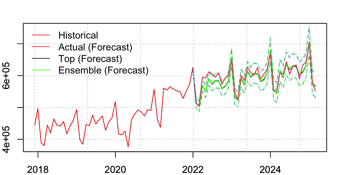
Code
par(opar)Note: You can overlay multiple predictive distributions using the add = TRUE argument in plot() for class tsmodel.distribution.
The following table compares performance metrics between the top model and the ensemble forecast. The ensemble consistently outperforms the top model across all metrics:
Code
tab <- rbind(tsmetrics(p_top, actual = test, alpha = 0.1),
             tsmetrics(p_ensemble, actual = test, alpha = 0.1))
rownames(tab) <- c("Top","Ensemble")
tab |> kable()| h | MAPE | MASE | MSLRE | BIAS | MIS | CRPS | |
|---|---|---|---|---|---|---|---|
| Top | 38 | 0.0209699 | 0.7469724 | 0.0006989 | -8584.579 | 84066.94 | 9169.592 |
| Ensemble | 38 | 0.0202501 | 0.7225133 | 0.0006459 | -7044.015 | 83491.41 | 8857.881 |
10.4 Conclusion
This demo showed how to apply automatic model selection with support for retaining the top N models and performing ensemble forecasting. By leveraging both predictive distributions and weighted ensembling, users can obtain more stable and accurate forecasts — particularly valuable when models are structurally similar but individually uncertain.
11 Demo: Variance Dynamics
In Section 19.2.2 of Hyndman et al. (2008), the authors illustrate an extension of the innovations state space model incorporating exponential GARCH dynamics. The appeal of the exponential GARCH model lies in its ability to ensure positivity of the variance without requiring parameter constraints.
In the tsissm package, we instead opt for the standard (vanilla) GARCH model, applying bounds on both the GARCH parameters and the overall persistence of the variance process. While this may initially appear more complex, it is actually simpler in practice—especially when accommodating non-Gaussian distributions. For example, using Johnson’s SU distribution complicates the calculation of the expected value of the absolute standardized innovations, which lacks a closed form and is required in the exponential GARCH model. With a standard GARCH structure, this complexity is avoided.
That said, the decision to include variance dynamics should be made with care. Many nominal economic time series that exhibit apparent heteroscedasticity become much more homoscedastic when deflated by the Consumer Price Index (CPI) or a similar price index. Moreover, structural breaks and transitory changes can mimic heteroscedastic behavior, misleading standard statistical tests into detecting heteroscedasticity when none is truly present.
11.1 SPY Closing Price
Heteroscedasticity in financial returns typically stems from volatility clustering, asymmetric responses to news, and shifting market conditions. These characteristics make GARCH-type models a natural choice in financial econometrics.
In this example, we model the adjusted closing prices of the S&P 500 ETF (SPY) using the innovations state space model. The specification includes:
- Log returns (\(\lambda = 0\))
- A random walk component
- AR dynamics
- GARCH(1,1) variance dynamics
- Johnson’s SU distribution for the residuals
We also account for structural level shifts, such as those occurring around the COVID-19 pandemic, by including them as regressors.
Code
data("spy", package = "tsissm")
y <- as.xts(spy)
xreg <- auto_regressors(y["2014/"], frequency = 1, lambda = 0, sampling = "days", method = "full",
                         check.rank = TRUE, discard.cval = 3.5, maxit.iloop = 10, maxit.oloop = 10, types = "LS")

exc <- which(xreg$xreg["2020-02-03"] == 1)
xreg$xreg <- xreg$xreg[,-exc]
xreg$init <- xreg$init[-exc]
We begin by estimating two models—one with constant variance, and one with time-varying (GARCH) variance:
Code
spec_constant <- issm_modelspec(y["2014/"], slope = FALSE, seasonal = FALSE, ar = 2, ma = 0, xreg = xreg$xreg,
                       lambda = 0, variance = "constant", distribution = "jsu")
spec_constant$parmatrix[grepl("^kappa", parameters), initial := xreg$init]
mod_constant <- estimate(spec_constant, scores = FALSE)

spec_dynamic <- issm_modelspec(y["2014/"], slope = TRUE, seasonal = FALSE, ar = 1, ma = 0, xreg = xreg$xreg,
                       lambda = 0, variance = "dynamic", distribution = "jsu")
spec_dynamic$parmatrix[grepl("^kappa",parameters), initial := xreg$init]
mod_dynamic <- estimate(spec_dynamic, scores = FALSE)
print(paste0("AIC(Dynamic): ", round(AIC(mod_dynamic),1)," | AIC(Constant): ", round(AIC(mod_constant),1)))
## [1] "AIC(Dynamic): 5059.5 | AIC(Constant): 5343.7"Based on the AIC values, the model with dynamic variance is preferred—even though it involves more parameters—demonstrating the usefulness of capturing volatility dynamics.
11.1.1 Model Summary
You can obtain a clean, professional summary of the estimated model using the as_flextable() method:
Code
mod_dynamic |> summary() |> as_flextable()Estimate | Std. Error | t value | Pr(>|t|) | ||
|---|---|---|---|---|---|
| 0.1949 | 0.0634 | 3.0736 | 0.0021 | ** |
| 0.0013 | 0.0005 | 2.5449 | 0.0109 | * |
| 0.7285 | 0.0742 | 9.8228 | 0.0000 | *** |
| -0.0398 | 0.0071 | -5.5796 | 0.0000 | *** |
| -0.0603 | 0.0140 | -4.2993 | 0.0000 | *** |
| -0.1387 | 0.0336 | -4.1331 | 0.0000 | *** |
| 0.0608 | 0.0300 | 2.0285 | 0.0425 | * |
| 0.0374 | 0.0269 | 1.3873 | 0.1654 | |
| -0.0587 | 0.0229 | -2.5633 | 0.0104 | * |
| 0.0549 | 0.0202 | 2.7171 | 0.0066 | ** |
| 0.0244 | 0.0188 | 1.2956 | 0.1951 | |
| -0.0612 | 0.0112 | -5.4834 | 0.0000 | *** |
| -0.0457 | 0.0155 | -2.9600 | 0.0031 | ** |
| -0.0489 | 0.0148 | -3.3034 | 0.0010 | *** |
| -0.0476 | 0.0097 | -4.9156 | 0.0000 | *** |
| 0.0488 | 0.0108 | 4.5240 | 0.0000 | *** |
| 0.1491 | 0.0165 | 9.0197 | 0.0000 | *** |
| 0.8337 | 0.0193 | 43.3078 | 0.0000 | *** |
| -0.8668 | 0.1687 | -5.1394 | 0.0000 | *** |
| 2.0636 | 0.1570 | 13.1431 | 0.0000 | *** |
Signif. codes: 0 '***' 0.001 '**' 0.01 '*' 0.05 '.' 0.1 ' ' 1 | |||||
sigma^2: 0.0001102 | |||||
LogLik: -5011.492 | |||||
AIC: 5059 | BIC: 1.021e+04 | |||||
DAC : 48 | MAPE : 0.71 | |||||
Model Equation | |||||
| |||||
| |||||
| |||||
| |||||
11.1.2 Visuals
The plot of the model components clearly displays the time-varying volatility typically associated with GARCH models:
Code
plot(mod_dynamic)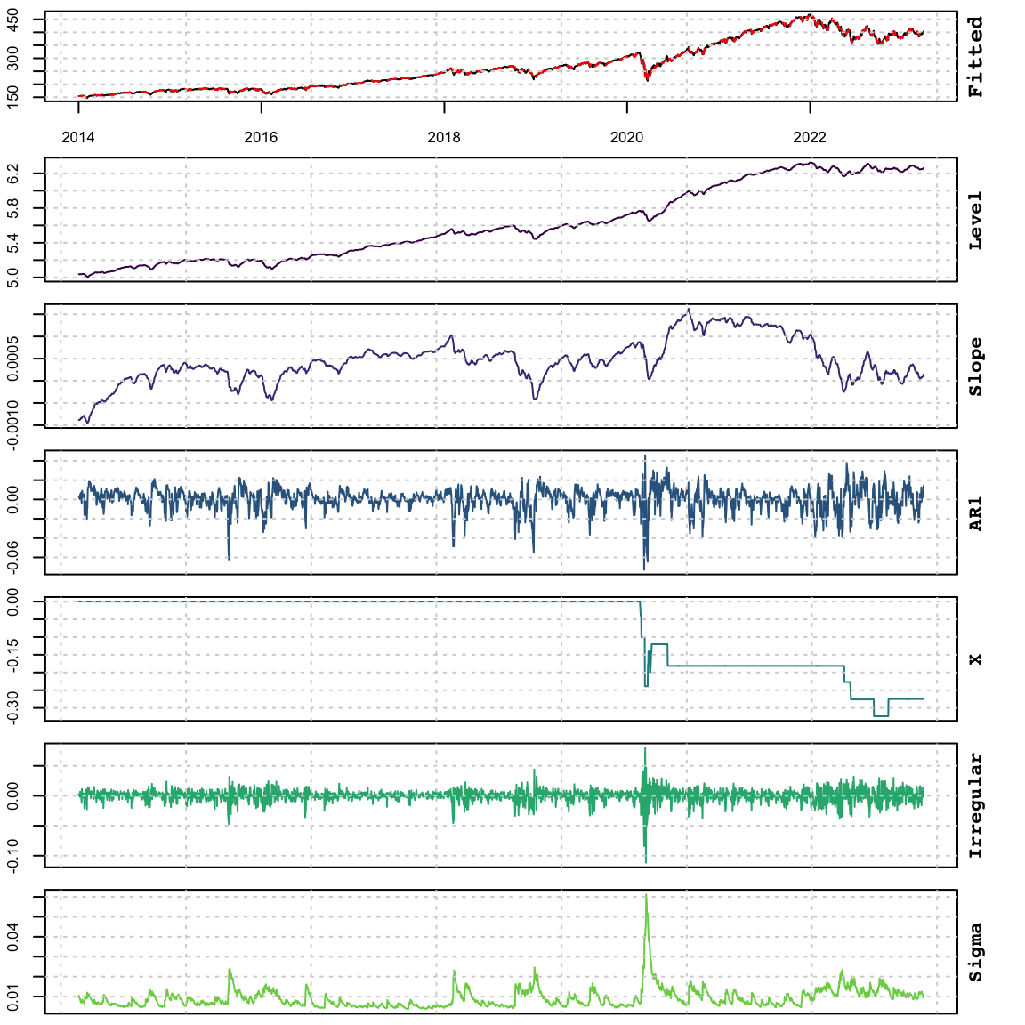
11.2 Conclusion
This demo showed how to model time-varying volatility using a financial time series example with the tsissm package. We showed how standard innovations state space models can be extended with GARCH dynamics and non-Gaussian distributions such as Johnson’s SU, allowing for more flexible modeling of conditional variance and fat-tailed behavior. This provides a robust framework for capturing some of the complexities of real-world time series, especially when volatility is an essential component of the dynamics.
12 Conclusion
The tsissm package makes use of the methods implemented in tsmethods and shared across all packages in the tsmodels framework. It provides an enhanced version of the tbats implementation in Hyndman et al. (2024), based on suggestions in Hyndman et al. (2008).
Future work may look at regularization of regressors, automatic anomaly handing and revision of the still experimental vector ETS (tsvets) package.
13 References
Anderson, B, and J Moore, 2012, Optimal Filtering (Dover Books on Electrical Engineering).
De Jong, Piet, 1991, The diffuse kalman filter, The Annals of Statistics 19, 1073–1083.
De Livera, Alysha M, Rob J Hyndman, and Ralph D Snyder, 2011, Forecasting time series with complex seasonal patterns using exponential smoothing, Journal of the American statistical association 106, 1513–1527.
Hyndman, Rob, George Athanasopoulos, Christoph Bergmeir, Gabriel Caceres, Leanne Chhay, Mitchell O’Hara-Wild, Fotios Petropoulos, Slava Razbash, Earo Wang, and Farah Yasmeen, 2024, forecast: Forecasting Functions for Time Series and Linear Models.
Hyndman, Rob, Anne B Koehler, J Keith Ord, and Ralph D Snyder, 2008, Forecasting with Exponential Smoothing: The State Space Approach.
Lütkepohl, Helmut, 2005, New Introduction to Multiple Time Series Analysis.
Footnotes
A future enhancement may incorporate regularization.↩︎
In our formulation we relax this to allow for other choices as well.↩︎
In the package, it is expected that the regression matrix is already pre-lagged.↩︎
The following equations apply for the case when all components are present (level, slope, seasonal and ARMA).↩︎
\(\lambda\) here should not be confused with the Box Cox lambda.↩︎
For \(j=1,\dots,k_i\) and \(i=1,\dots,T\), representing the number of harmonics \(k\) per seasonal period \(i\).↩︎
For simplicity of exposition, \(y_t\) is equivalent to \(y_t^{(\lambda)}\).↩︎
RTMB instead of TMB was used for the constraint due to issues discussed here.↩︎
In practice we could have just imposed the constraint on the first eigenvalue, but since D is non-symmetric, we have no guarantees, from what I have read, that the LAPACK routine (
dgeev) will always return the eigenvalues in decreasing order by modulus.↩︎We make use of the sandwich package by exporting
estfunandbreadmethods.↩︎Because the transformed residuals may be in different scales (different Box-Cox \(\lambda\)), include outliers, etc, we adopt the approach of first calculating the dependence using Kendall’s tau and then transform to Pearson’s correlation.↩︎