1 Introduction
The tsmarch package represents a re-write and re-think of the models in rmgarch. It is written using simpler S3 methods and classes, has a cleaner code base, extensive documentation and unit tests, provides speed gains by making use of parallelization in both R (via the future package) and in the C++ code (via RcppParallel package), and works with the new univariate GARCH package tsgarch.
To simplify usage, similar to the approach adopted in tsgarch, conditional mean dynamics are not included. Since the distributions are location/scale invariant, the series can be pre-filtered for conditional mean dynamics before submitting the data, but there is an option to pass the conditional_mean (cond_mean) as an argument during estimation, filtering, prediction and simulation so that it is incorporated into the output of various methods at each step of the way. Alternatively, the user can location shift (re-center) the simulated predictive distribution matrix by the pre-calculated conditional mean forecast, or pass the zero mean correlated predictive distribution innovations as an input to the conditional mean prediction simulation dynamics.
The nature of the models implemented allows for separable dynamics in estimation which means that individual series have univariate dynamics which can be estimated in parallel. However, the drawback to this1 is that for standard errors a partitioned Hessian must be calculated which may be very time consuming. While the package defaults to the use of OPG (outer of product of gradients) for standard errors which is fast, there is always the option to calculate the full partitioned Hessian for other types of standard error estimators.
The next sections provide a detailed overview of each of the 3 models available, namely the Dynamic Correlation GARCH model of Engle (2002) (DCC), the Copula-DCC model (see Patton (2009) and Ausin and Lopes (2010)) (CGARCH) and the Generalized Orthogonal GARCH model with multivariate affine Generalized Hyperbolic Distribution (see Chen, Härdle, and Spokoiny (2010) and Broda and Paolella (2009)) (GOGARCH).
2 Covariance Decomposition Models
The covariance decomposition type models decompose the dynamics of the conditional covariance into the conditional standard deviations and correlations, so that they may be expressed in such a way that the univariate and multivariate dynamics may be separated, thus simplifying the estimation process. This decomposition allows a great deal of flexibility by defining individual univariate dynamics for each of the margins, and separate dynamics for the conditional correlation, using a 2-stage estimation process.
2.1 Constant Correlation
In the Constant Conditional Correlation (CCC) model of Bollerslev (1990) the equation for the conditional covariance can be represented as:
\[ H_t = D_t R D_t = \rho_{ij}\sqrt{h_{iit}h_{jjt}}, \tag{1}\]
where \(D_t = diag(\sqrt {h_{11,t}},\ldots,\sqrt{h_{nn,t}})\), and \(R\) is the positive definite constant correlation matrix.
The conditional variances, \(h_{ii,t}\), which can be estimated separately, usually admit some type of GARCH(p,q) model, but can be generalized to any other admissible model.
The conditions for the positivity of the covariance matrix \(H_t\) are that \(R\) is positive definite and the diagonal elements of \(D_t\), \(h_{ii,t}\), are positive.
Formally, the model may be represented as follow:
\[ \begin{aligned} y_{t}&=\mu_{t}+\varepsilon_{t},\varepsilon_{t}\sim N\left({0,\Sigma_{t}}\right)\\ \Sigma_{t}&=D_{t}RD_{t}\\ z_{t}&=D_{t}^{-1}\varepsilon_{t}\\ LL_{t}\left(\theta\right)&=\frac{1}{2}\left(n \log\left(2\pi\right)+2\log\left|D_t\right|+\log\left|R\right|+z'_tR^{-1}z_t\right) \end{aligned} \tag{2}\]
where \(y_t\) is a vector representing the series values at time \(t\), \(\mu_t\) a vector of the conditional mean at time t for each series, \(\varepsilon_t\) a vector of zero mean residuals which have a multivariate normal distribution with conditional covariance \(\Sigma_t\), and \(LL_t\left(\theta\right)\) is the log-likelihood at time \(t\) given a parameter vector \(\theta\) of univariate GARCH (or other model) parameters. The constant correlation matrix \(R\) is usually approximated by its sample counterpart as
\[ R = \frac{1}{T}\sum\limits_{t=1}^{T}{z_t z_t'} \]
where \(z_t\) is the vector of GARCH standardized residuals at time \(t\).
2.2 Dynamic Conditional Correlation
Allowing the correlation to be time varying, whilst retaining the 2-stage separation of dynamics, creates an additional challenge to the positive definiteness constraint at each point in time for the conditional correlation. Engle (2002) proposed the following proxy process :
\[ \begin{aligned} Q_t &= \bar Q + \sum\limits_{j=1}^{q}{a_j\left(z_{t-j}z'_{t-j}-\bar Q\right)} + \sum\limits_{j=1}^{p}{b_j\left(Q_{t-j}-\bar Q\right)}\\ &= \left(1 - \sum\limits_{j=1}^{q}{a_j} - \sum\limits_{j=1}^{p}{b_j}\right)\bar Q + \sum\limits_{j=1}^{q}{a_j\left(z_{t-j}z'_{t-j}\right)} + \sum\limits_{j=1}^{p}{b_j Q_{t-j}} \end{aligned} \tag{3}\]
where \(a_j\) and \(b_j\) are non-negative coefficients with the constraint that they sum to less than 1 for stationarity and positive definiteness, and \(\bar Q\) is the unconditional matrix of the standardized residuals \(z_t\). To recover \(R_t\), the following re-scaling operation is performed:
\[ R_t = \text{diag}\left(Q_t\right)^{-1/2}Q_t\text{diag}\left(Q_t\right)^{-1/2} \tag{4}\]
Under the assumption that \(\varepsilon_t\sim N\left(0,\Sigma_t\right)\), the log-likelihood is:
\[ \begin{aligned} LL_t\left(\theta\right) &= \frac{1}{2}\left(\log\left(2\pi\right) + 2\log\left|D_t\right| + z_t z'_t\right) - \frac{1}{2}\left(z_t z'_t + \log\left|R_t\right| + z'_t R^{-1}_t z_t\right)\\ &= LL_{V,t}(\phi) + LL_{R,t}\left(\psi|\phi\right) \end{aligned} \tag{5}\]
where \(LL_{V,t}(\phi)\) is the log-likelihood of the conditional variances given the GARCH parameters \(\phi\), and \(LL_{R,t}\left(\psi|\phi\right)\) is the log-likelihood of the conditional correlation given the DCC parameters \(\psi|\phi\) (conditioned on the GARCH parameters).
2.3 Estimation
Estimation of the CCC and DCC models is done in 2 steps. The first step is to estimate the conditional variances for each series using a univariate GARCH model. The conditional variances are then used to standardize the residuals which are then used to estimate the conditional correlation matrix. Since the first step is separable, it can be done in parallel for each series.2
2.4 Standard Errors
Since estimation is performed in 2 stages, the log-likelihood is the sum of these 2 stages. More specifically, the second stage log-likelihood is estimated conditioning on the parameters of the first stage. Details of the assumptions behind this and the arguments for the asymptotic distribution of the estimates are put forth in Engle and Sheppard (2001), who posit that the asymptotic distribution of the 2-stage DCC model estimates with parameters \(\theta = \left(\phi, \psi\right)\) is:
\[ \sqrt{T}\left(\hat\theta_T - \hat\theta_0\right) \overset{\text{A}}{\sim} {N\left(0, B^{-1}_0 M_0 {B'}^{-1}_0\right)}\\ \tag{6}\]
where:
\[ B_0 = \begin{bmatrix} \nabla_{\phi\phi} \ln f_1(\phi_0) & 0 \\ \nabla_{\phi\psi} \ln f_2(\phi_0) & \nabla_{\psi\psi} \ln f_2(\theta_0) \end{bmatrix} = \begin{bmatrix} B_{11} & 0 \\ B_{12} & B_{22} \end{bmatrix} \tag{7}\]
and
\[ M_0 = \text{var} \left[ \sum_{t=1}^{T} \left\{ T^{-1/2} \nabla_{\phi}' \ln f_1(r_t, \phi_0), T^{-1/2} \nabla_{\psi}' \ln f_2(r_t, \phi_0, \psi_0) \right\} \right] = \begin{bmatrix} M_{11} & M_{12} \\ M_{12} & M_{22} \end{bmatrix} \tag{8}\]
where \(B_0^{-1}\) and \(M_0\) are the Hessian and the covariance matrix of the score vector respectively, also called the bread and meat of the sandwich estimator. In the case of this 2 stage estimation procedure, the Hessian is partitioned into 4 blocks, \(B_{11}\), \(B_{12}\), \(B_{22}\) and \(M_{11}\), \(M_{12}\), \(M_{22}\), where \(B_{11}\) and \(M_{11}\) are the Hessian and covariance matrix of the first stage log-likelihood, and \(B_{22}\) and \(M_{22}\) are the Hessian and covariance matrix of the second stage log-likelihood. \(B_{12}\) and \(M_{12}\) are the cross derivatives of the first and second stage log-likelihoods.
Because the Hessian is partitioned, the calculation of the standard errors is more computationally intensive than the standard OPG (outer product of gradients) method. While the package defaults to the OPG method, the user can choose to calculate the full partitioned Hessian during estimation, for which parallel functionality has been implemented to provide some speed gains. The package uses numerical derivatives for the second stage estimation, as well as the for calculation of the standard errors. When the partitioned Hessian is present, a number of additional estimators become available including the those of the QML and HAC (using the bandwidth of Newey and West (1994)) type.
2.5 Distributions
The original DCC model was based on the assumption that the residuals are normally distributed, as shown in Equation 2 and Equation 5.
However, this is not always the case in practice. There are 2 possible approaches to this problem. The first is to use a different multivariate distribution for the DCC model and the second is to use the Copula approach.
2.5.1 Multivariate Student Distribution
Introducing a multivariate distribution which requires estimation of higher moment parameters implies that the univariate margins must also have the same distribution and usually the same higher moment parameters. This in turn implies the need for joint estimation of all dynamics in the model with specific constraints on the joint parameters. This is computationally intensive and may not be feasible for anything but a few series. However, it may be possible to estimate the higher moment parameters using QML (quasi-maximum likelihood) for the first stage (essentially use a normal distribution for the residuals), and then use these estimates in the second stage estimation. This is the approach taken in the tsmarch package (similar to Bauwens and Laurent (2005)), when using the multivariate Student distribution with log-likelihood equal to:
\[ \begin{aligned} LL_t\left(\theta, \nu| \phi\right) & = \log\Gamma\left(\frac{\nu + n}{2}\right) - \log\Gamma\left(\frac{\nu}{2}\right) -\frac{n}{2}\log\left(\pi\left(\nu - 2\right)\right)\\ &- \frac{1}{2}\log\left|R_t\right| - \log\left|D_t\right| - \frac{\nu + 2}{2}\log\left(1 + \frac{1}{\nu-2}z_t' R_t^{-1} z_t\right) \end{aligned} \tag{9}\]
where \(\nu\) is the degrees of freedom parameter of the Student distribution, and \(n\) is the number of series. The assumption post-estimation is that the marginal distribution of each series is Student with the same degrees of freedom parameter \(\nu\).
2.5.2 Copula Distribution (cgarch)
The Copula approach is a more general approach which allows for the use of different marginal distributions for each series. In simple terms, the Copula is a function which links the marginal distributions to the joint distribution by applying a transformation to the marginal residuals to make them uniformly distributed. The joint distribution is then obtained by applying the inverse distribution of the Copula to the uniform margins
Specifically:
\[ \begin{aligned} u_t & = C\left(F_1\left(z_{1,t}\right),\ldots,F_n\left(z_{n,t}\right)\right)\\ \epsilon_t & = F^{-1}\left(u_t\right) \end{aligned} \tag{10}\]
where \(F\) is the marginal distribution function, \(F^{-1}\) is the inverse of the multivariate distribution function, \(C\) is the Copula function, and \(u_t\) is the vector of uniform margins. The transformation of the margins is called the Probability Integral Transform (PIT). There are a number of ways to transform the margins to uniform distributions, including a parametric transform (also called the Inference-Functions-For-Margins by Joe (1997)), using the empirical CDF (also called pseudo-likelihood and investigated by Genest, Ghoudi, and Rivest (1995)) and the semi-parametric approach (see Davison and Smith (1990)). All three approaches are implemented in the tsmarch package. The package implements both a Normal and Student Copula, with either constant or dynamic correlation. For the Student Copula, the log-likelihood is given by:
\[ \begin{aligned} LL_t\left(\theta\right) & = \sum\limits_{i=1}^{n} \left( -\frac{1}{2} \log h_{i,t} + \log f_{i,t}(z_{i,t}) \right) + \log c_t\left(u_{i,t},\ldots, u_{n,t}\right)\\ & = LL_{V,t}\left(\phi\right) + LL_{R,t}\left(\psi,\eta|\phi\right) \end{aligned} \tag{11}\]
where
\[ \log c_t\left(u_{1,t}, \ldots, u_{n,t}\right) = \log f_t\left(F_i^{-1}\left(u_{1,t}|\eta\right), \ldots, F_i^{-1}\left(u_{n,t}|\eta\right) | R_t,\eta \right) - \sum\limits_{i=1}^{n} \log f_i\left( F_i^{-1}(u_{i,t})|\eta \right) \tag{12}\]
with \(u_{i,t} = F_{i,t}\left(\varepsilon_{i,t}|\phi_i \right)\) is the PIT transformation of each series by it’s conditional distribution estimated in the first stage GARCH process by any choice of dynamics and distributions, \(F_i^{-1}\left(u_{i,t}|\eta\right)\) represents the quantile transformation of the uniform margins subject to a common shape parameter of the multivariate Student Copula, and \(f_t\left( F_i^{-1}\left(u_{1,t}|\eta\right), \ldots, F_i^{-1}\left(u_{n,t}|\eta\right) | R_t,\eta \right)\) is the joint density of the Student Copula with shape parameter \(\eta\) and correlation matrix \(R_t\).
Therefore, the log-likelihood is composed of essentially 3 parts: the first stage univariate models, the univariate PIT transformation and inversion given the Copula distribution and the second stage multivariate model.
The correlation can be modeled as either constant or dynamic in the Copula model. The dynamic correlation is modeled in the same way as the DCC model, but the residuals undergo a transformation prior to estimation of the correlation. Appendix Section 7.1 provides a more detailed overview for the constant correlation case.
Essentially, the difference between the standard DCC type model and the one with a Copula distribution involves the PIT transformation step, which is reflected in the inference (standard errors), forecasting and simulation methods for this model.
2.6 Generalized Dynamics
A number of extensions to the DCC model have been proposed in the literature. These include the use of asymmetric and generalized dynamics. Cappiello, Engle, and Sheppard (2006) generalize the DCC model with the introduction of the Asymmetric Generalized DCC (AGDCC) where the dynamics of \(Q_t\) now become:
\[ Q_t = \left(\bar Q - A'\bar Q A - B'\bar Q B - G'\bar N G\right) + \sum\limits_{j=1}^{q}{A'_j z_{t-j}z'_{t-j}A_j} + \sum\limits_{j=1}^{q}{G'_j{\bar z}_{t-j}{\bar z}'_{t-j}G_j} + \sum\limits_{j=1}^{p}{B'_j Q B_j} \tag{13}\]
where A, B and G are the \(N\times N\) parameter matrices, \(\bar z_t\) are the zero-threshold standardized residuals (equal to \(z_t\) when less than zero else zero otherwise), \(\bar Q\) and \(\bar N\) are the unconditional matrices of \(z_t\) and \(\bar z_t\) respectively. The generalization allows for cross dynamics between the standardized residuals, and cross-asymmetric dynamics. However, this comes at the cost of increased computational complexity making it less feasible for large scale systems. Additionally, covariance targeting in such a high dimensional system where the parameters are no longer scalars creates difficulties in imposing positive definiteness constraints. The tsmarch package does not implement this generalized model, but instead a scalar version to capture asymmetric dynamics (adcc):
\[ Q_t = \left(1 - \sum\limits_{j=1}^{q}{a_j} - \sum\limits_{j=1}^{p}{b_j}\right)\bar Q - \sum\limits_{j=1}^{q}{g_j}\bar N + \sum\limits_{j=1}^{q}{a_j\left(z_{t-k}z'_{t-j}\right)} + \sum\limits_{j=1}^{q}{g_j\left(\bar z_{t-k}\bar z'_{t-j}\right)} + \sum\limits_{j=1}^{p}{b_j Q_{t-j}} \tag{14}\]
2.7 Forecasting and Simulation
Because of the non linearity of the DCC evolution process, the multi-step ahead forecast of the correlation cannot be directly solved. Engle and Sheppard (2001) provide a couple of suggestions which form a reasonable approximation. In the tsmarch package we instead use a simulation approach, similar to the other packages in the tsmodels universe, and in doing so generate a simulated distribution of the h-step ahead correlation and covariance. This also generalizes to the copula model which does not have a closed form solution. Formally, for a draw \(s\) at time \(t\), the simulated correlation is given by:
\[ \begin{aligned} Q^s_t & = \bar Q + \sum\limits_{j=1}^{q}{a_j\left(z^s_{t-j}{z^s}'_{t-j}-\bar Q\right)} + \sum\limits_{j=1}^{p}{b_j\left({Q^s}_{t-j}-\bar Q\right)}\\ R^s_t & = \text{diag}\left({Q^s}_t\right)^{-1/2}{Q^s}_t\text{diag}\left({Q^s}\right)^{-1/2}\\ z^s_t & = E \Lambda^{1/2} {\epsilon^s}_t \end{aligned} \tag{15}\]
where \({\epsilon^s}_t\) is a vector of standard Normal random variables, \(\Lambda\) is the diagonal matrix of the eigenvalues of \({R^s}_t\) and \(E\) is the matrix of eigenvectors of \({R^s}_t\), such that:
\[ {R^s}_t = E \Lambda E' \tag{16}\]
For the multivariate Student distribution, the draws for \(z_t\) are generated as :
\[ z^s_t = E \Lambda^{1/2} {\epsilon^s}_t \sqrt{\frac{\nu}{W^s}} \tag{17}\]
where \(W\) is a random variable from a chi-squared distribution with \(\nu\) degrees of freedom. For \({\epsilon^s}_t\), it is also possible to instead use the empirical standardized and de-correlated residuals, an option which is offered in the package.
2.8 Weighted Distribution
Since all predictions are generated through simulation, the weighted predictive distribution \(\bar {y_t}^s\) can be obtained as:
\[ \bar {y_t}^s|w = \sum\limits_{i=1}^{n} w_{i,t} {y_{i,t}}^s \tag{18}\]
where \(s\) is a sample draw from the simulated predictive distribution of the \(n\) series, and \(w_{i,t}\) the weight on series \(i\) at time \(t\).
2.9 News Impact Surface
Engle and Ng (1993) introduced the news impact curve as a tool for evaluating the effects of news on the conditional variances, which was further extended by Kroner and Ng (1998) to the multivariate GARCH case. The news impact surface shows the effect of shocks from a pair of assets on their conditional covariance (or correlation). Formally, the correlation \(R_{i,j}\) given a set of shock \(\left(z_i,z_j\right)\) is given by:
\[ R_{i,j}\left(z_i,z_j\right) = \frac{\left(1 - a - b\right)\bar{Q}_{i,j} - g\bar N_{i,j} + a z_{i} z_{j} + g \bar z_{i}\bar z_{j} + b \bar Q_{i,j}}{\sqrt{\left[\left(1 - a - b\right)\bar{Q}_{i,i} - g\bar N_{i,i} + a z_{i}^2 + g \bar z_{i}^2 + b \bar Q_{i,i}\right] \cdot \left[\left(1 - a - b\right)\bar{Q}_{j,j} - g\bar N_{i,j} + a z_{j}^2 + g \bar z_{j}^2 + b \bar Q_{j,j}\right]}} \tag{19}\]
where \(\bar z\), \(\bar Q\) and \(\bar N\) are defined as in Equation 13.
2.10 Critique
The DCC model has come under a considerable amount of criticism in the literature, particularly by Caporin and McAleer (2008) who argue that consistency and asymptotic Normality of the estimators has not been fully established, and instead proposed the indirect DCC model (essentially a scalar BEKK) which models directly the conditional covariance matrix and forgoes univariate GARCH dynamics.
Aielli (2013) also points out that the estimation of \(Q_t\) as the empirical counterpart of the correlation matrix of \(z_t\) is inconsistent since \(E\left[z_t z'_t\right] = E\left[R_t\right] \neq E\left[Q_t\right]\). They propose a corrected DCC (cDCC) model which includes a corrective step which eliminates this inconsistency, albeit at the cost of targeting which is not allowed.
3 Generalized Orthogonal GARCH Model (gogarch)
The GOGARCH model in the tsmarch package is based on the approach described in Chen, Härdle, and Spokoiny (2010), Broda and Paolella (2009) and Ghalanos, Rossi, and Urga (2015). Unlike the covariance decomposition models, the Generalized Orthogonal GARCH model is akin to a full distributional decomposition model rather than just the covariance, since it makes use of higher moments to achieve independent margins from which univariate models can then be used to estimate the conditional dynamics (see Schmidt, Hrycej, and Stützle (2006) for details on the multivariate affine Generalized Hyperbolic distribution).
Formally, the stationary return series \(y_t\) follows a linear dynamic model:
\[ \begin{aligned} y_t &= \mu_t + \varepsilon_t\\ \varepsilon_t &= A f_t\\ \end{aligned} \tag{20}\]
where \(A\) is an invertible and constant mixing matrix, which transforms the independent components \(f_t\) back into the residuals \(\varepsilon_t\). This can be further decomposed into de-whitening and rotation matrices, \(\Sigma^{1/2}\) and \(U\) respectively:
\[ A = \Sigma^{1/2}U \tag{21}\]
where \(\Sigma\) is the unconditional covariance matrix of the residuals and performs the role of de-correlating (whitening) the residuals prior to rotation (independence). It is at this juncture where dimensionality reduction may also be performed, by selecting the first \(m\) principal components of the residuals. In that case \(\varepsilon_t \approx \hat \varepsilon_t = A f_t\) since the dimensionality reduced system only approximates the original residuals.
The rotation matrix \(U\) is calculated through the use of Independent Component Analysis (ICA) which is a method separating multivariate mixed signals into additive statistically independent and non-Gaussian components3 (see Hyvärinen and Oja (2000)). There are 2 choices of ICA algorithms in the tsmarch package: one based on the RADICAL algorithm of Learned-Miller and Fisher (2003) which uses an efficient entropy estimator (due to Vasicek (1976)) which is robust to outliers and requires no strong characterization assumptions about the data generating process.4 and one based on the FASTICA algorithm of Hyvarinen (1999).
The independent components \(f_t\) can be further decomposed as:
\[ f_t = H_t^{1/2} z_t \tag{22}\]
where \(H_t\) is the conditional covariance matrix of the independent components with \(H_t = E[f_t f_t' | \mathfrak{F}_{t-1}]\), being a diagonal matrix with elements \((h_{1,t},\ldots,h_{n,t} )\) which are the conditional variances of the factors, and \(z_t = (z_{1,t},\ldots,z_{n,t})'\). The random variable \(z_{i,t}\) is independent of \(z_{jt-s}\) \(\forall j \neq i\) and \(\forall s\), with \(E[z_{i,t}|\mathfrak{F}_{t-1}]=0\) and \(E[z_{i,t}^2]=1\), implying that \(E[f_t|\mathfrak{F}_{t-1}] = \mathbf{0}\) and \(E[\varepsilon_t|\mathfrak{F}_{t-1}] = \mathbf{0}\). The factor conditional variances, \(h_{i,t}\) can be modeled as a GARCH-type process. The unconditional distribution of the factors is characterized by:
\[ E[f_t] = \mathbf{0} \quad E[f_t f'_t] = I_n \tag{23}\]
which, in turn, implies that:
\[ E[\varepsilon_t] = \mathbf{0} \quad E[\varepsilon_t\varepsilon'_t] = A A'. \tag{24}\]
It then follows that the return series can be expressed as:
\[ y_t = \mu_t + A H_t^{1/2} z_t. \tag{25}\]
The conditional covariance matrix, \(\Sigma_t \equiv E[(y_t -\mu_t)(y_t - \mu_t)'|\mathfrak{F}_{t-1}]\) is given by \(\Sigma_t = A H_t A'\).
The Orthogonal Factor model of Alexander (2002)5 which uses only information in the covariance matrix, leads to uncorrelated components but not necessarily independent unless assuming a multivariate normal distribution. However, while whitening is not sufficient for independence, it is nevertheless an important step in the pre-processing of the data in the search for independent factors, since by exhausting the second order information contained in the covariance matrix it makes it easier to infer higher order information, reducing the problem to one of rotation (orthogonalization).
3.1 Estimation
The estimation of the GOGARCH model is performed in 3 steps.
- Filter the data for conditional mean dynamics (\(\mu_{i,t}\)). Similar to the DCC model, this is performed outside the system.
- Perform Independent Component Analysis (ICA) on the residuals to separate out the additive and statistically independent components.
- Estimate the conditional distribution of each independent component using an admissible univariate model. In the
tsmarchpackage we use thetsgarchpackage for estimating the GARCH model for each factor with either a Generalized Hyperbolic (gh) or Normal Inverse Gaussian (nig) distribution.6
The log-likelihood of the GOGARCH model is composed of the individual log-likelihoods of the univariate independent factor GARCH models and a term for the mixing matrix:
\[ LL_t\left(\theta, A\right) = \log\left|A^{-1}\right| + \sum\limits_{i=1}^{n} \log\left(GH_{\lambda_i}\left(\theta_i\right)\right) \tag{26}\]
where \(GH_{\lambda_i}\) is the Generalized Hyperbolic distribution with shape parameter \(\lambda_i\) for the \(i\)-th factor. Since the inverse of the mixing matrix is the un-mixing matrix \(A^{-1} = W = K'U\), and since the determinant of \(U\) is 1 (\(|U|=1\)), the the log-likelihood simplifies to:
\[ LL_t\left(\theta, A\right) = \log\left|K\right| + \sum\limits_{i=1}^{n} \log\left(GH_{\lambda_i}\left(\theta_i\right)\right) \tag{27}\]
In the presence of dimensionality reduction, \(K\) is no longer square, and we cannot directly compute its determinant. Instead, we use the determinant of \(K K'\) , to reflect the combined effect of whitening and dimensionality reduction:
\[ LL_t\left(\theta, A\right) = \log\left|K K'\right| + \sum\limits_{i=1}^{m} \log\left(GH_{\lambda_i}\left(\theta_i\right)\right) \tag{28}\]
A key advantage of this approach is the ability to estimate multivariate dynamics using only univariate methods, providing for feasible estimation of large scale systems. The speed advantage of this approach does not come for free, as there is a corresponding need for memory to handle the parallelization offered, particularly when generating higher co-moment matrices.
3.2 Co-Moments
The linear affine representation of the GOGARCH model provides for a closed-form expression for the conditional co-moments. The first 3 co-moments are given by:
\[ \begin{aligned} M^2_t &= A M^2_{f,t} A'\\ M^3_t &= A M^3_{f,t} \left(A' \otimes A'\right)\\ M^4_t &= A M^4_{f,t} \left(A' \otimes A' \otimes A'\right) \end{aligned} \tag{29}\]
where \(M_{f,t}^2\), \(M_{f,t}^3\) and \(M_{f,t}^4\) are the \((N \times N)\) conditional covariance, \((N \times N^2)\) the conditional third co-moment matrix and the \((N \times N^3)\) conditional fourth co-moment matrix of the factors, respectively, represented as unfolded tensors7
These are calculated from the univariate factor dynamics, and defined as:
\[ M_{f,t}^3 = \begin{bmatrix} M_{1,f,t}^3, M_{2,f,t}^3, \ldots, M_{n,f,t}^3 \end{bmatrix} \tag{30}\]
\[ M_{f,t}^4 = \begin{bmatrix} M_{1,1,f,t}^4, M_{1,2,f,t}^4, \ldots, M_{1,n,f,t}^4 \, | \, \ldots \, | \, M_{n,1,f,t}^4, M_{n,2,f,t}^4, \ldots, M_{n,n,f,t}^4 \end{bmatrix} \tag{31}\]
where \(M_{k,f,t}^3, k=1,\ldots,n\) and \(M_{k,l,f,t}^4, k,l=1,\ldots,n\) are the \(N\times N\) sub-matrices of \(M_{f,t}^3\) and \(M_{f,t}^4\), respectively, with elements
\[ \begin{aligned} m_{i,j,k,f,t}^3 & = & E[f_{i,t}f_{j,t}f_{k,t}|\mathfrak{F}_{t-1}] \\ m_{i,j,k,l,f,t}^4 & = & E[f_{i,t}f_{j,t}f_{k,t}f_{l,t}|\mathfrak{F}_{t-1}]. \end{aligned} \tag{32}\]
Since the factors \(f_{i,t}\) can be decomposed as \(z_{i,t}\sqrt{h_{i,t}}\), and given the assumptions on \(z_{i,t}\) then \(E[f_{i,t}f_{j,t}f_{k,t}|\mathfrak{F}_{t-1}] = 0\). It is also true that for \(i \neq j\neq k \neq l\) \(E[f_{i,t}f_{j,t}f_{k,t}f_{l,t}|\mathfrak{F}_{t-1}] = 0\) and when \(i=j\) and \(k=l\),
\[ E[f_{i,t}f_{j,t}f_{k,t}f_{l,t}|\mathfrak{F}_{t-1}] = h_{i,t}^2 h_{k,t}^2. \tag{33}\]
Thus, under the assumption of mutual independence, all elements in the conditional co-moments matrices with at least 3 different indices are zero. Finally, standardizing the conditional co-moments one obtains conditional co-skewness and co-kurtosis of \(y_t\),
\[ \begin{aligned} S_{i,j,k,t} &= \frac{m_{i,j,k,t}^3}{({\sigma_{i,t}}{\sigma_{j,t}}{\sigma _{k,t}})}, \\ K_{i,j,k,l,t} &= \frac{m_{i,j,k,l,t}^4}{({\sigma_{i,t}}{\sigma_{j,t}}{\sigma_{k,t}}{\sigma _{l,t}})} \end{aligned} \tag{34}\]
where \(S_{i,j,k,t}\) represents the series co-skewness between elements \(i,j,k\) of \(y_t\), \(\sigma_{i,t}\) the standard deviation of \(y_{i,t}\), and in the case of \(i=j=k\) represents the skewness of series \(i\) at time \(t\), and similarly for the co-kurtosis tensor \(K_{i,j,k,l,t}\). Two natural applications of return co-moments matrices are Taylor type utility expansions in portfolio allocation and higher moment news impact surfaces.
The weighted moments are calculated as follows:
\[ \begin{aligned} \mu_{1,t} &= w_t` M^1_{t}\\ \mu_{2,t} &= w_t' M^2_{t} w_t\\ \mu_{3,t} &= w_t' M^3_{t} \left(w_t \otimes w_t\right)\\ \mu_{4,t} &= w_t' M^4_{t} \left(w_t \otimes w_t \otimes w_t\right)\\ \end{aligned} \tag{35}\]
where \(w_t\) is the vector of weights at time \(t\). Using the vectorization operator \(vec\) the weighted moments can be re-written compactly as:
\[ \mu_k = \text{vec}\left(M_k\right)'\underbrace{(w_t \otimes \ldots \otimes w_t)}_{k \text{ times}} \tag{36}\]
One application of this is in the calculation of the Constant Absolute Risk Aversion utility function, using a Taylor series expansion as in Ghalanos, Rossi, and Urga (2015):
\[ E_{t-1}\left[U\left(W_t\right)\right] = E_{t-1}\left[-\exp\left(-\eta \bar W_t\right)\right] \approx -\exp\left(-\eta \bar W_t\right)\left[1 + \frac{\eta}{2}\mu_{2,t} - \frac{\eta^3}{3!}\mu_{3,t} + \frac{\eta^4}{4!}\mu_{4,t}\right] \tag{37}\]
where \(\eta\) represents the investor’s constant absolute risk aversion, with higher (lower) values representing higher (lower) aversion, and \(\bar W_t = w'_t E_{t-1}\left[y_t\right]\) is the expected portfolio return at time \(t\). Note that this approximation includes two moments more than the mean-variance criterion, with the skewness and kurtosis are directly related to investor preferences (dislike) for odd (even) moments, under certain mild assumptions given in Scott and Horvath (1980).
3.3 Weighted Distribution
The weighted conditional density of the model may be obtained via the inversion of the Generalized Hyperbolic characteristic function through the fast fourier transform (FFT) method as in Chen, Härdle, and Spokoiny (2010) or by simulation. The tsmarch package generates both simulated predictive distributions as well as the weighted \(p^*\), \(d^*\) and \(q^*\) distribution functions based on FFT.
It should be noted that while the n-dimensional NIG distribution is closed under convolution, when the distributional higher moment parameters are allowed to be different across assets, as is the case here, this property no longer holds which is why we adopt the FFT method.
Provided that \(\epsilon_t\) is a n-dimensional vector of innovations, marginally distributed as 1-dimensional standardized GH, the density of weighted asset returns, \(w_{i,t}y_{i,t}\) is:
\[ w_{i,t}y_{i,t} - w_{i,t}\mu_{i,t} = \bar w_{i,t}\epsilon_{i,t}\sim \text{maGH}_{\lambda_i}\left(\bar w_{i,t}\bar\mu_{i,t},\left|\bar w_{i,t}\delta_{i,t}\right|,\frac{\alpha_{i,t}}{\left|\bar w_{i,t}\right|}, \frac{\beta_{i,t}}{\left|\bar w_{i,t}\right|} \right) \tag{38}\]
where \(\bar w_{t} = w'_tAH^{1/2}_t\) and hence \(\bar w_{i,t}\) is the \(i\)-th element of this vector, \(\mu_{i,t}\) is the conditional mean of series \(i\) at time \(t\), and the parameter vector \(\left(\bar \mu_{i,t}, \delta_{i,t}, \beta_{i,t}, \alpha_{i,t}, \lambda_i\right)\) represents the generalized hyperbolic distributional parameters which have been converted from their \(\left(\rho,\zeta\right)\) parameterization used in the tsgarch package estimation routine. In order to obtain the weighted density we need to sum the individual log densities of \(\epsilon_{i,t}\):
\[ \varphi(u) = \prod\limits_{i = 1}^n {\varphi_{\bar w{\epsilon_i}}} (u) = \exp{ \left( \text{i}u\sum\limits_{j = 1}^d \bar\mu_j + \sum\limits_{j = 1}^d \left( \frac{\lambda_j}{2} \log{\left(\frac{\gamma}{\upsilon}\right)} + \log \left(\frac{K_{\lambda_j}(\bar\delta_j\sqrt{\upsilon})}{K_{\lambda_j}(\bar\delta_j \sqrt{\gamma})} \right) \right) \right) } \tag{39}\]
where, \(\gamma = \bar \alpha_j^2 - \bar \beta_j^2\), \(\upsilon = \bar \alpha_j^2 - {({\bar \beta_j} + {\text{i}}u)^2}\), and \((\bar \alpha_j, \bar \beta_j, \bar \delta_j, \bar \mu_j)\) are the scaled versions of the parameters \((\alpha_{i}, \beta_{i}, \delta_{i}, \mu_{i})\) as shown in Equation 38. The density may be accurately approximated by FFT as follows:
\[ {f_y}(r) = \frac{1}{2\pi}\int_{-\infty}^{+\infty}{{e^{( - \text{i}u r)}}} \varphi_y (u)\mathrm{d}u \approx \frac{1}{2\pi}\int_{ - s}^s {{e^{( - \text{i}u r)}}} \varphi_y (u)\mathrm{d}u. \tag{40}\]
Once the density is obtained, we use smooth approximations to obtain functions for the density (\(d^*\)), quantile (\(q^*\)) and distribution (\(p^*\)), with random number generation provided by the use of the inverse transform method using the quantile function.
3.4 Factor News Impact Surface
Consider the equation for the construction of the conditional covariance matrix \(\Sigma_t\):
\[ \Sigma_t = A H_t A' \]
where \(H_t\) is the diagonal conditional covariance matrix of the independent components. The factor news impact covariance surface is a measure of the effect of shocks from the independent factors on the conditional covariance of the returns of assets \(i\) and \(j\) at time \(t-1\). In order to construct this we first generate the news impact curves for all the factors using a common grid of shock values, and then calculate the effect of these on the conditional covariance of the returns of assets \(i\) and \(j\). Since the factors are independent, we simply loop through all pairwise combinations of these shocks8 to calculate the covariance surface, keeping the value of the other factors constant:
\[ \Sigma_{i,j} = a_{k,i} \cdot h_{k,k}|\epsilon_k \cdot a_{k,j} + a_{l,i} \cdot h_{l,l}|\epsilon_l \cdot a_{l,j} + \sum_{\substack{m=1 \\ m \neq k, l}}^{n} a_{m,i} \cdot h_{m,m}|{\epsilon_m=0} \cdot a_{m,j} \tag{41}\]
where :
- \(a_{k,i}\) is the loading of factor \(k\) on asset \(i\),
- \(h_{k,k}|\epsilon_k\) is the conditional variance of factor \(k\) from the news impact curve given the shock \(\epsilon_k\),
- \(a_{k,i} \cdot h_{k,k}|\epsilon_k \cdot a_{k,j}\) captures the contribution of factor k to the covariance between assets i and j, based on the shock \(\epsilon_k\)
applied to factor \(k\), - \(a_{l,i} \cdot h_{l,l}|\epsilon_l \cdot a_{l,j}\) captures the contribution of factor \(l\) to the covariance between assets i and j, based on the shock \(\epsilon_l\) applied to factor l and
- \(\sum_{\substack{m=1 \\ m \neq k, l}}^{n} a_{m,i} \cdot s_{m,m}(0) \cdot a_{m,j}\) captures the contributions of all other factors (except k and l), where their variances are held constant at their unconditional levels (i.e., with no shocks).
This means that the covariance will be affected by both the relative sign and magnitude of the loadings and the relative magnitude of the variance of the factors.
The news impact surface is not restricted to the covariance matrix, but can be extended to the conditional co-skewness and co-kurtosis, but that is only truly meaningful when the higher moment distributional parameters are allowed to vary as in Ghalanos, Rossi, and Urga (2015).
4 Methods and Classes
Figures Figure 1 and Figure 2 provide a visual summary of the main methods in the package for the DCC and GOGARCH type models. Blue boxes denote a method which produces a custom class which can be further manipulated with other methods9, whilst Appendix Section 7.2 provides a summary of some of the methods and output classes in the tsmarch package and the type of parallelization they use.
5 Demo
The following sections provide a short demo on the 3 models in the package. The blog may in the future include additional applications.
For all demos we’ll use the globalindices dataset which consists of a selection of the log weekly returns (Friday) of 34 global financial indices from Yahoo Finance starting on 1991-12-13 and ending on 2024-06-21. For the demo we choose the following 12 indices:
- North America
- SPX (S&P 500 Index – United States)
- NDQ (NASDAQ Composite Index – United States)
- SNX (S&P SmallCap 600 Index – United States)
- TSX (S&P/TSX Composite Index – Canada)
- Europe
- CAC (CAC 40 Index – France)
- DAX (DAX 30 Index – Germany)
- AEX (Amsterdam Exchange Index – Netherlands)
- UKX (FTSE 100 Index – United Kingdom)
- Asia
- HSI (Hang Seng Index – Hong Kong)
- NKX (Nikkei 225 Index – Japan)
- STI (Straits Times Index – Singapore)
- KOSPI (Korea Composite Stock Price Index – South Korea)
The training data spans the period 1991-12-31/2022-08-05 (1600 data points), leaving the period from 2022-08-12/2024-06-21 (98 data points) for evaluation.
We use the same conditional mean dynamics across demos, consisting of an AR(6) model for each series. In practice one would use a more sophisticated approach but for this demo this will suffice.
Code
data("globalindices")
globalindices <- as.xts(globalindices)
tickers <- c("SPX","NDQ","SNX","TSX","CAC","DAX","AEX","UKX","HSI","NKX","STI","KOSPI")
regions <- c(rep("NORTH_AMERICA",4),rep("EUROPE",4),rep("ASIA",4))
train_set <- globalindices["/2022-08-05", tickers]
test_set <- globalindices["2022-08-12/", tickers]
5.1 Conditional Mean Dynamics
We first estimate the conditional mean model as well as rolling 1-step ahead forecasts based on a rolling scheme to filter new information (rather than re-estimating), as well as an unconditional 98-step ahead forecast, which we’ll make use in the next sections.
Code
cond_mean_model <- lapply(1:12, function(i){
  train_set[,i] |> arma_modelspec(order = c(6,0)) |> estimate()
})

.fitted <- do.call(cbind, lapply(cond_mean_model, function(x) {
  unname(as.numeric(fitted(x)))
}))
.fitted <- xts(.fitted, index(train_set))
colnames(.fitted) <- colnames(train_set)

.residuals <- do.call(cbind, lapply(cond_mean_model, function(x) {
  unname(as.numeric(residuals(x)))
}))
.residuals <- xts(.residuals, index(train_set))
colnames(.residuals) <- colnames(train_set)


.filtered <- lapply(1:12, function(i) {
    tmp <- do.call(rbind, lapply(1:98, function(j) {
        filtered_model <- cond_mean_model[[i]] |> tsfilter(y = test_set[1:j,i])
        filtered_residuals <- tail(residuals(filtered_model), 1)
        filtered_mean <- tail(fitted(filtered_model), 1)
        cbind(filtered_mean, filtered_residuals)
      }))
    return(tmp)
})

.filtered_mean <- do.call(cbind, lapply(.filtered, function(x) x[,1]))
.filtered_residuals <- do.call(cbind, lapply(.filtered, function(x) x[,2]))
colnames(.filtered_mean) <- colnames(train_set)
colnames(.filtered_residuals) <- colnames(train_set)

.predicted <- do.call(cbind, lapply(1:12, function(i) {
    do.call(rbind, lapply(0:97, function(j) {
      if (j == 0) {
        predict(cond_mean_model[[i]], h = 1)$mean
      } else {
        cond_mean_model[[i]] |> tsfilter(y = test_set[1:j,i]) |> predict(h = 1) |> {\(x) x$mean}()
      }
    }))
}))
colnames(.predicted) <- colnames(train_set)

.uncforecast <- do.call(cbind, lapply(1:12, function(i) {
  cond_mean_model[[i]] |> predict(h = 98) |> {\(x) x$mean}()
}))
colnames(.uncforecast) <- colnames(train_set)
For the DCC and CGARCH models we also need to pre-estimate the univariate GARCH models prior to passing them to the multivariate model specification. This allows for more flexibility in how to structure the univariate dynamics for each series. We pass the zero mean residuals from the AR model we previously estimated:
Code
garch_model <- lapply(1:12, function(i){
  .residuals[,i] |> garch_modelspec(model = "egarch", constant = FALSE) |> estimate(keep_tmb = TRUE)
})
garch_model <- to_multi_estimate(garch_model)
names(garch_model) <- colnames(train_set)
Notice that for estimation we set the argument keep_tmb to TRUE. This is critical for use in the multivariate models. Also notice that the returned object from the call to the to_multi_estimate is a validated list of univariate GARCH models. However, as of writing this, there is an additional step required which is naming the list with the series names. This will be fixed in a later version so that it is done automatically.
5.2 DCC Model
5.2.1 Estimation
We use an asymmetric DCC model with multivariate Student distribution, estimated in the first stage using Quasi Maximum Likelihood (QML). Note that we are passing the estimated conditional mean from the AR(6) model to the DCC specification. This is optional, but takes care of re-centering any relevant output by the conditional mean instead of having the user do this manually.
Code
dcc_spec <- dcc_modelspec(garch_model, cond_mean = .fitted, dcc_order = c(1,1), dynamics = "adcc", distribution = "mvt")
dcc_model <- estimate(dcc_spec)
summary(dcc_model)
## DCC Model Summary
## DCC Dynamics: ADCC | MVT
## Coefficients:
## Estimate Std. Error t value Pr(>|t|)
## alpha_1 7.188e-03 7.002e-04 10.266 < 2e-16 ***
## gamma_1 2.694e-03 9.742e-04 2.765 0.00568 **
## beta_1 9.875e-01 1.059e-03 932.048 < 2e-16 ***
## shape 1.094e+01 6.921e-01 15.811 < 2e-16 ***
## ---
## Signif. codes: 0 '***' 0.001 '**' 0.01 '*' 0.05 '.' 0.1 ' ' 1
##
## N: 1600 | Series: 12
## LogLik: 51995.6, AIC: -103863, BIC: -103519The time varying covariance and correlation can be extracted using the tscov and tscor methods respectively. There is also a plot function for this estimated object which provides a heat map of the pairwise correlations over time:
Code
plot(dcc_model)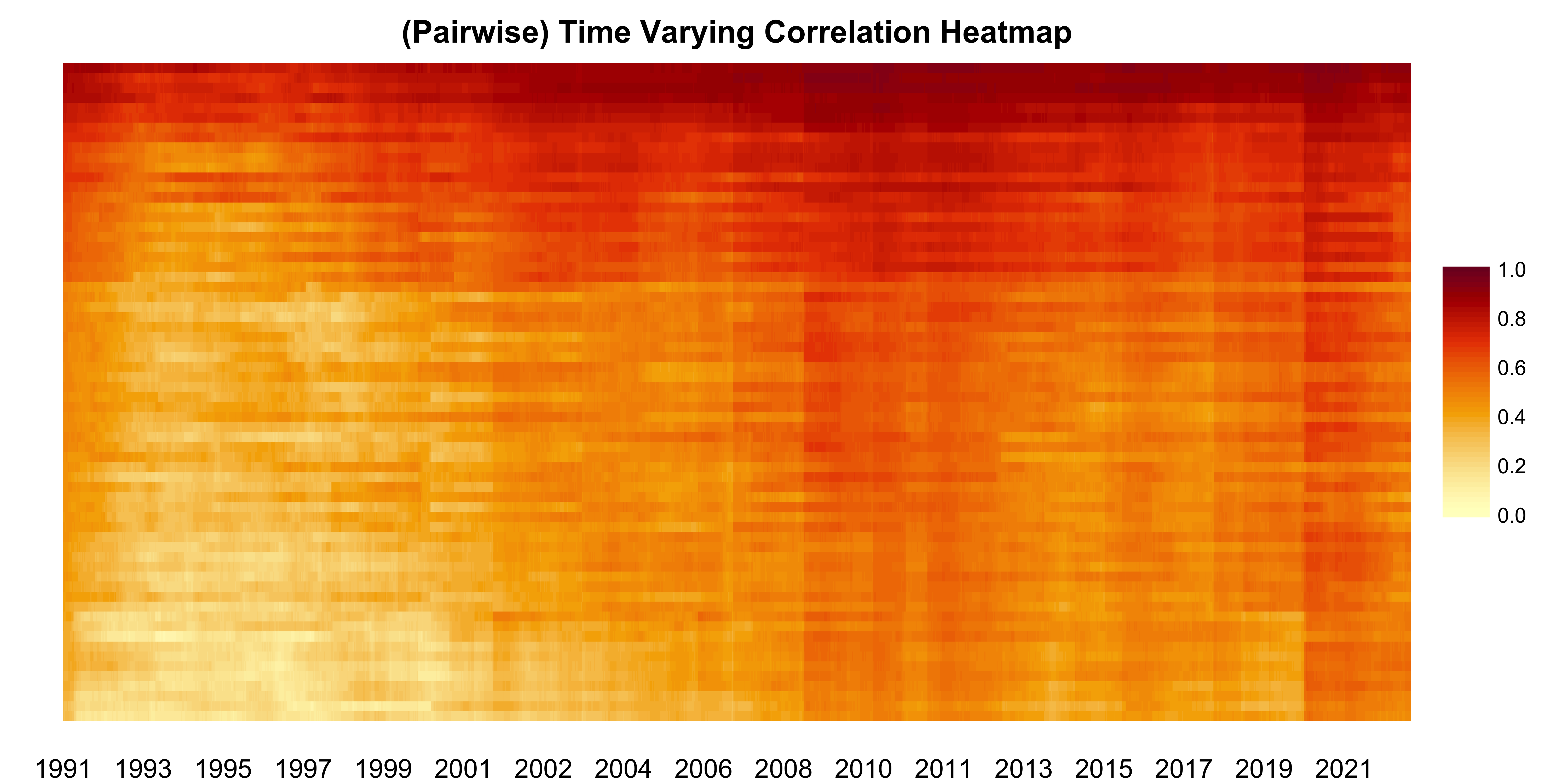
The interesting observation we can make is that around 2008 and late 2019 the pairwise correlations across all indices (i.e. across regions) spiked, indicating the perceived increase in global risk.
We can also plot the newsimpact surface for pairwise combinations:
Code
newsimpact(dcc_model, type = "correlation", pair = c(1,2)) |> plot()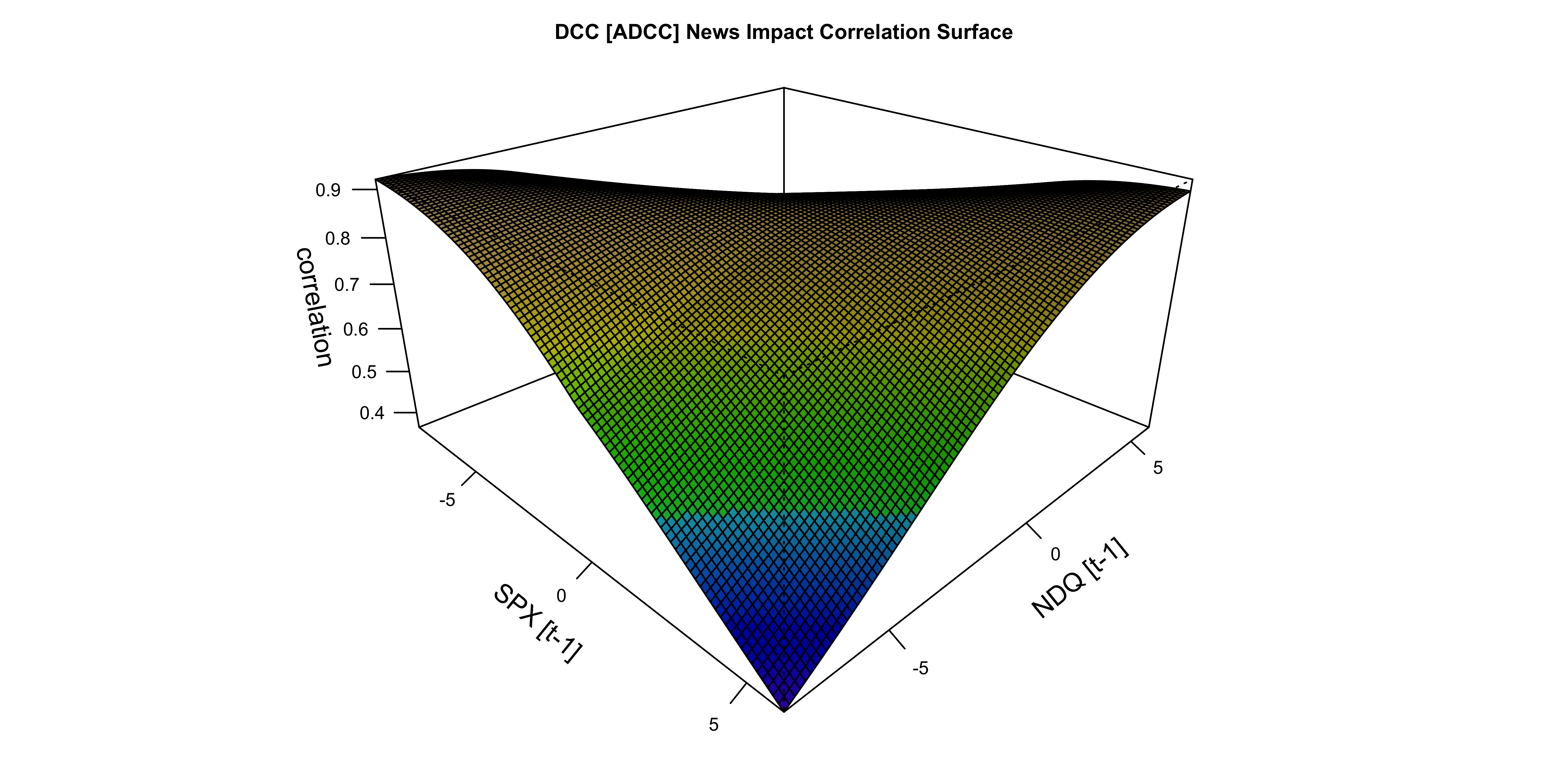
5.2.2 Prediction
The next step is to generate a rolling 1-step ahead forecast of the value at risk for the testing period. We follow the same approach as in the conditional mean model by filtering the existing model with updated information and then generating a 1-step ahead prediction, which is a quick way to backtest without having to re-estimate the coefficients. We use an equal weighted vector for creating the portfolio.
Let’s unpack the steps:
- For the first prediction we use the already estimated DCC model estimated up to time T and pass the already predicted conditional mean for T+1 (
predicted[1,]). - In the next step, we update the DCC model with new information at time T+1 (
.filtered_residuals[1,]) which consists of the already pre-filtered residuals and fitted values from the conditional mean model. - We then predict for T+2|T+1 and also pass the predicted conditional mean values for time T+2 (
.predicted[2,]). - Finally, we calculate the value at risk from the weighted simulated distribution given a set of equal weights using the
value_at_riskmethod on the predicted object.
Code
w <- rep(1/12, 12)
value_risk <- sapply(0:97, function(i){
  if (i == 0) {
    p <- dcc_model |> predict(h = 1, nsim = 5000, seed = 100, cond_mean = .predicted[1,]) |> value_at_risk(weights = w, alpha = 0.05)
  } else {
    p <- dcc_model |> tsfilter(y = .filtered_residuals[1:i,], cond_mean = .filtered_mean[1:i,]) |> predict(h = 1, cond_mean = .predicted[i + 1,], nsim = 5000, seed = 100) |> value_at_risk(weights = w, alpha = 0.05)
  }
  return(p)
})
value_risk <- xts(value_risk, index(test_set))
actual <- xts(coredata(test_set) %*% w, index(test_set))
as_flextable(var_cp_test(actual, value_risk, 0.05), signif.stars = TRUE, include.decision = TRUE)
Test | DoF | Statistic | Pr(>Chisq) | Decision(5%) | |
|---|---|---|---|---|---|
Kupiec (UC) | 1 | 0.8948 | 0.3442 | Fail to Reject H0 | |
CP (CCI) | 1 | 0.1915 | 0.6617 | Fail to Reject H0 | |
CP (CC) | 2 | 1.0863 | 0.5809 | Fail to Reject H0 | |
CP (D) | 1 | 9.4692 | 0.0021 | ** | Reject H0 |
Signif. codes: 0 '***' 0.001 '**' 0.01 '*' 0.05 '.' 0.1 ' ' 1 | |||||
Coverage: 0.05, Obs: 98, Failures: 3, E[Failures]: 4 | |||||
Hypothesis(H0) : Unconditional(UC), Independent(CCI), Joint Coverage(CC) and Duration(D) | |||||
The table shows the output of the var_cp_test from the tstests package, where we find that with the exception of the conditional duration test, all other tests appear to indicate that the model performed well for the 5% quantile level.
Finally, we show an alternative way to predict, in this case for the long run forecast:
Code
p_1 <- dcc_model |> predict(h = 98, nsim = 5000, seed = 100, cond_mean = .uncforecast)
# without centering, so that we get zero mean residuals
p_2 <- dcc_model |> predict(h = 98, nsim = 5000, seed = 100)
simulated_res <- p_2$mu
arma_simulated_prediction <- lapply(1:12, function(i){
  tmp <- predict(cond_mean_model[[i]], h = 98, innov_type = "r", innov = t(simulated_res[,i,]), nsim = 5000, forc_dates = index(test_set))
  tmp <- tmp$distribution
  return(tmp)
})
In the first case we passed the predicted mean to the predict function which then re-centers the simulated predictive distribution by this. In the second case we predict the DCC model without the cond_mean input in order to get back just the zero mean simulated and correlated residuals which we then pass to the prediction method of the ARMA model which then uses these in the predictive simulation.
We can inspect the output visually for a couple of series:
Code
par(mfrow = c(2,1), mar = c(2,2,2,2))
plot(arma_simulated_prediction[[1]], main = "SPX Forecast Distribution", gradient_color = "white")
dcc_distribution <- t(p_1$mu[,1,])
colnames(dcc_distribution) <- colnames(arma_simulated_prediction[[1]])
class(dcc_distribution) <- "tsmodel.distribution"
plot(dcc_distribution, add = TRUE, median_color = "red", gradient_color = "white", interval_color = "red")

plot(arma_simulated_prediction[[10]], main = "NKX Forecast Distribution", gradient_color = "white")
dcc_distribution <- t(p_1$mu[,10,])
colnames(dcc_distribution) <- colnames(arma_simulated_prediction[[10]])
class(dcc_distribution) <- "tsmodel.distribution"
plot(dcc_distribution, add = TRUE, median_color = "red", gradient_color = "white", interval_color = "red")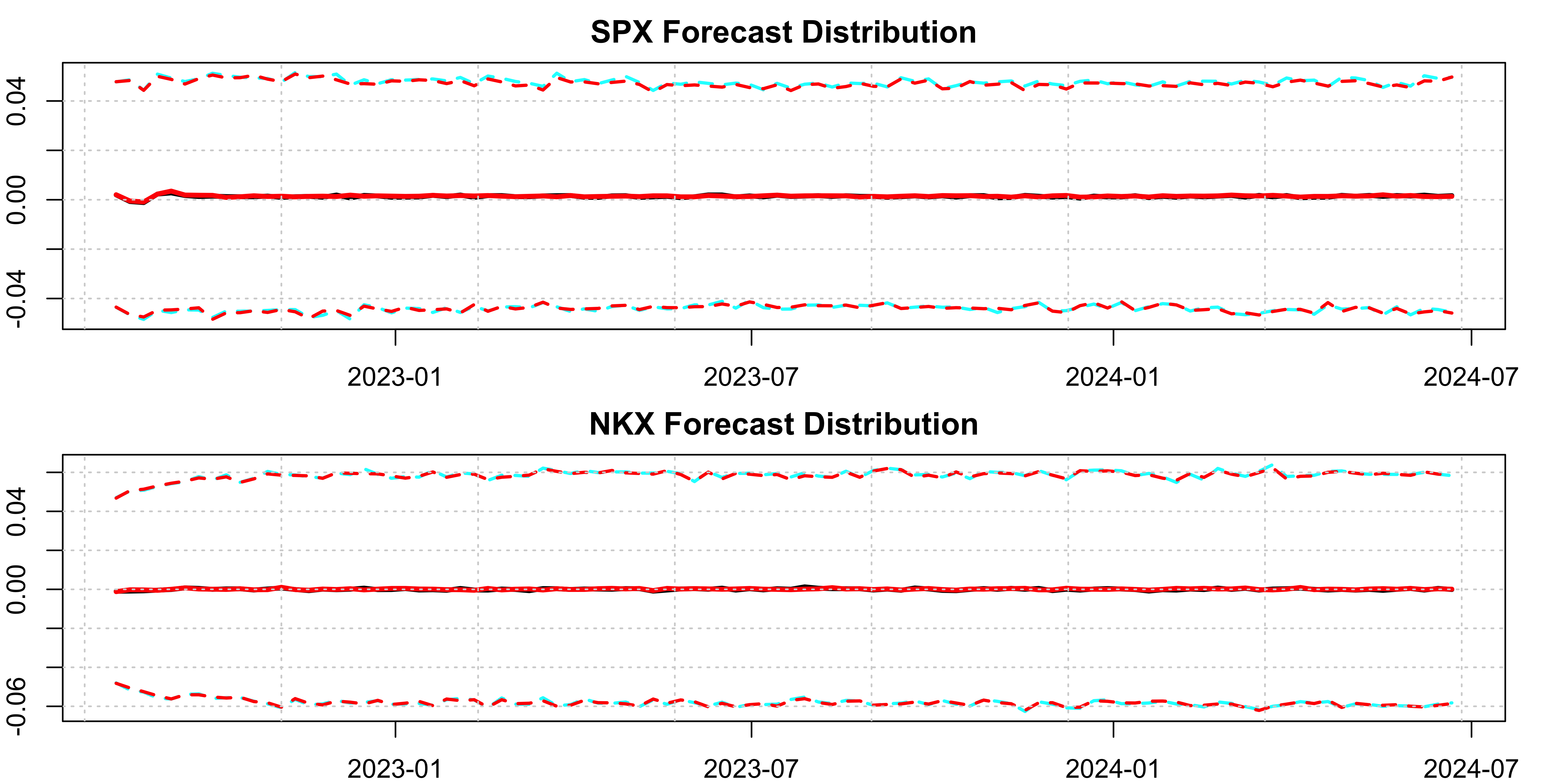
We can also form the value at risk of the weighted portfolio to check the correlation.
Code
# we re-center to the exact mean since we also do this for the DCC model distribution
arma_simulated_prediction <- lapply(1:12, function(i){
  d <- arma_simulated_prediction[[i]]
  d <- scale(d, scale = FALSE, center = TRUE)
  d <- scale(d, scale = FALSE, center = -as.numeric(.uncforecast[,i]))
  return(d)
})
arma_multi_correlated <- array(unlist(arma_simulated_prediction), dim = c(5000, 98, 12))
arma_multi_correlated <- aperm(arma_multi_correlated, perm = c(2, 3, 1))

v_1 <- do.call(cbind, lapply(1:98, function(i){
  t(arma_multi_correlated[i,,]) %*% w
}))
v_2 <- do.call(cbind, lapply(1:98, function(i){
  t(p_1$mu[i,,]) %*% w
}))
plot(apply(v_1, 2, quantile, 0.05), type = "l", ylab = "VaR 5%", xlab = "")
lines(apply(v_2, 2, quantile, 0.05), col = "orange", lty = 2, lwd = 2)
legend("topright", c("ARMA Prediction with DCC correlated residuals","DCC Prediction with ARMA conditional mean recentering"), col = c("black","orange"), lty = c(1,2), lwd = c(1,2), bty = "n")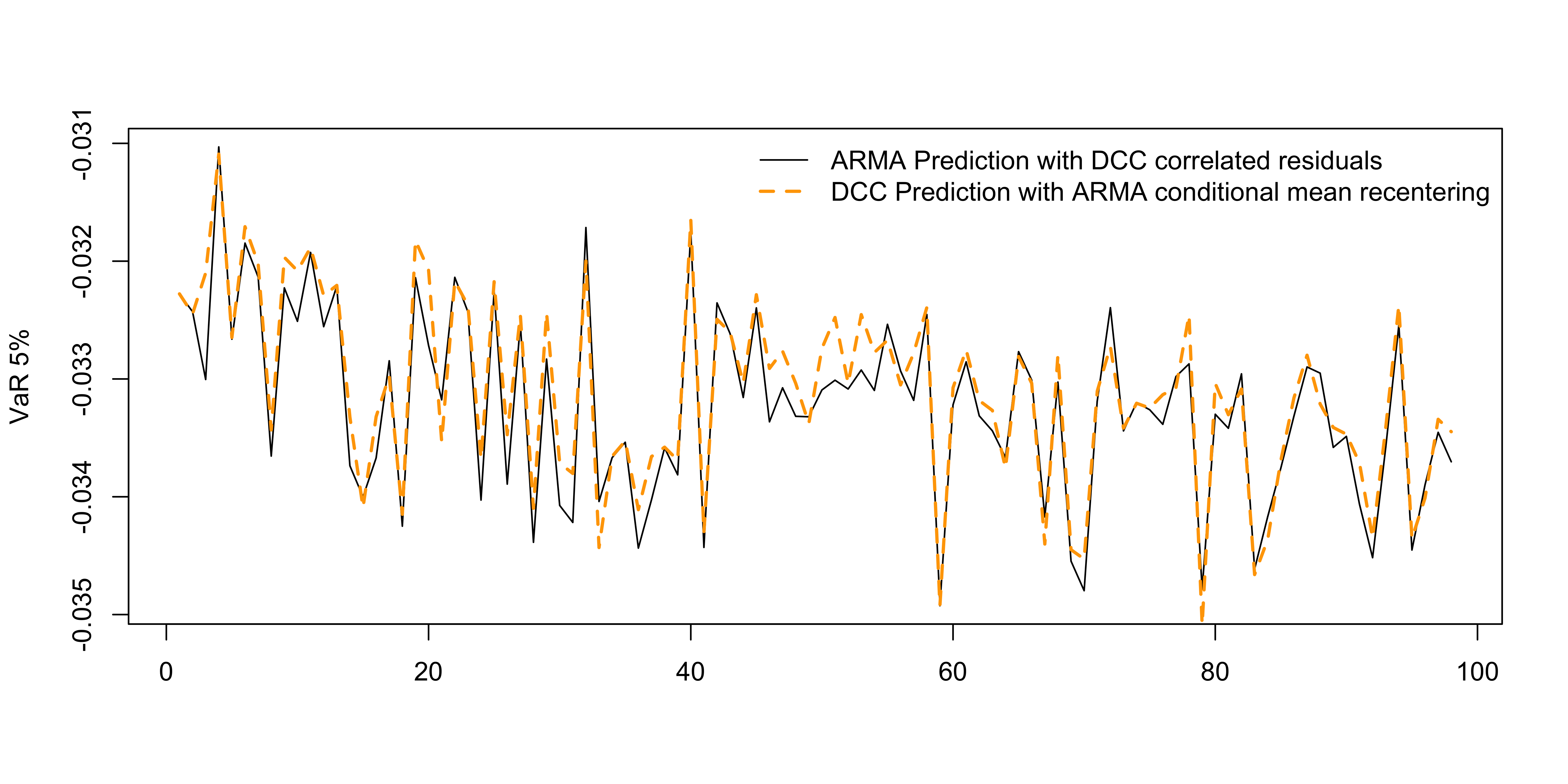
We observe that the two approaches to predicting the conditional mean with the DCC model are almost identical. The second method where the simulated innovations are passed to the conditional mean model is usually preferred, but not all functions have the option of generating either a predictive distribution or allowing one to pass a matrix of simulated innovations. In that case, the first approach of re-centering the predictive distribution from the DCC model should form a very good approximation.
5.2.3 Other Methods
The correlation and covariance methods are respectively called tscor and tscov, from the tsmethods package. In the case of a prediction or simulated object, these are usually [n x n x h x nsim] arrays, but there is an argument called distribution which averages these across all simulation draws (nsim).
Similarly, the tsaggregate methods returns a list of the simulated mean and variance of the weighted portfolio which is also a simulated distribution for the prediction and simulated objects unless the user sets distribution to FALSE.
The value_at_risk and expected_shortfall methods operate on predicted or simulated objects calculating the respective value at risk and expected shortfall measures on these simulated distributions. These methods are currently created in the tsmarch package but may be eventually moved to a separate tsrisk package.
5.3 Copula GARCH Model
5.3.1 Estimation
We follow the same approach as in the DCC model to estimate the Copula GARCH model, but calculate a new set of univariate GARCH models with Jonhson’s SU (jsu) margins.
Code
garch_model_jsu <- lapply(1:12, function(i){
  .residuals[,i] |> garch_modelspec(model = "egarch", distribution = "jsu", constant = FALSE) |> estimate(keep_tmb = TRUE)
})
garch_model_jsu <- to_multi_estimate(garch_model_jsu)
names(garch_model_jsu) <- colnames(train_set)

cgarch_spec <- cgarch_modelspec(garch_model_jsu, cond_mean = .fitted, dcc_order = c(1,1), dynamics = "adcc",
                                transformation = "parametric", copula = "mvt")
cgarch_model <- estimate(cgarch_spec)
summary(cgarch_model)
## CGARCH Model Summary
## Copula Dynamics: parametric | MVT | ADCC
## Coefficients:
## Estimate Std. Error t value Pr(>|t|)
## alpha_1 6.723e-03 5.885e-04 11.423 < 2e-16 ***
## gamma_1 6.381e-03 1.030e-03 6.196 5.79e-10 ***
## beta_1 9.873e-01 9.727e-04 1015.042 < 2e-16 ***
## shape 1.821e+01 1.465e+00 12.427 < 2e-16 ***
## ---
## Signif. codes: 0 '***' 0.001 '**' 0.01 '*' 0.05 '.' 0.1 ' ' 1
##
## N: 1600 | Series: 12
## LogLik: 52093.6, AIC: -104011, BIC: -103538Notice that the shape parameter is much higher than that of the DCC model estimated in the previous demo (i.e. less leptokurtic). This is because most of the extreme tails where captured in the first stage dynamics.
Code
newsimpact(cgarch_model, type = "correlation", pair = c(1,2)) |> plot()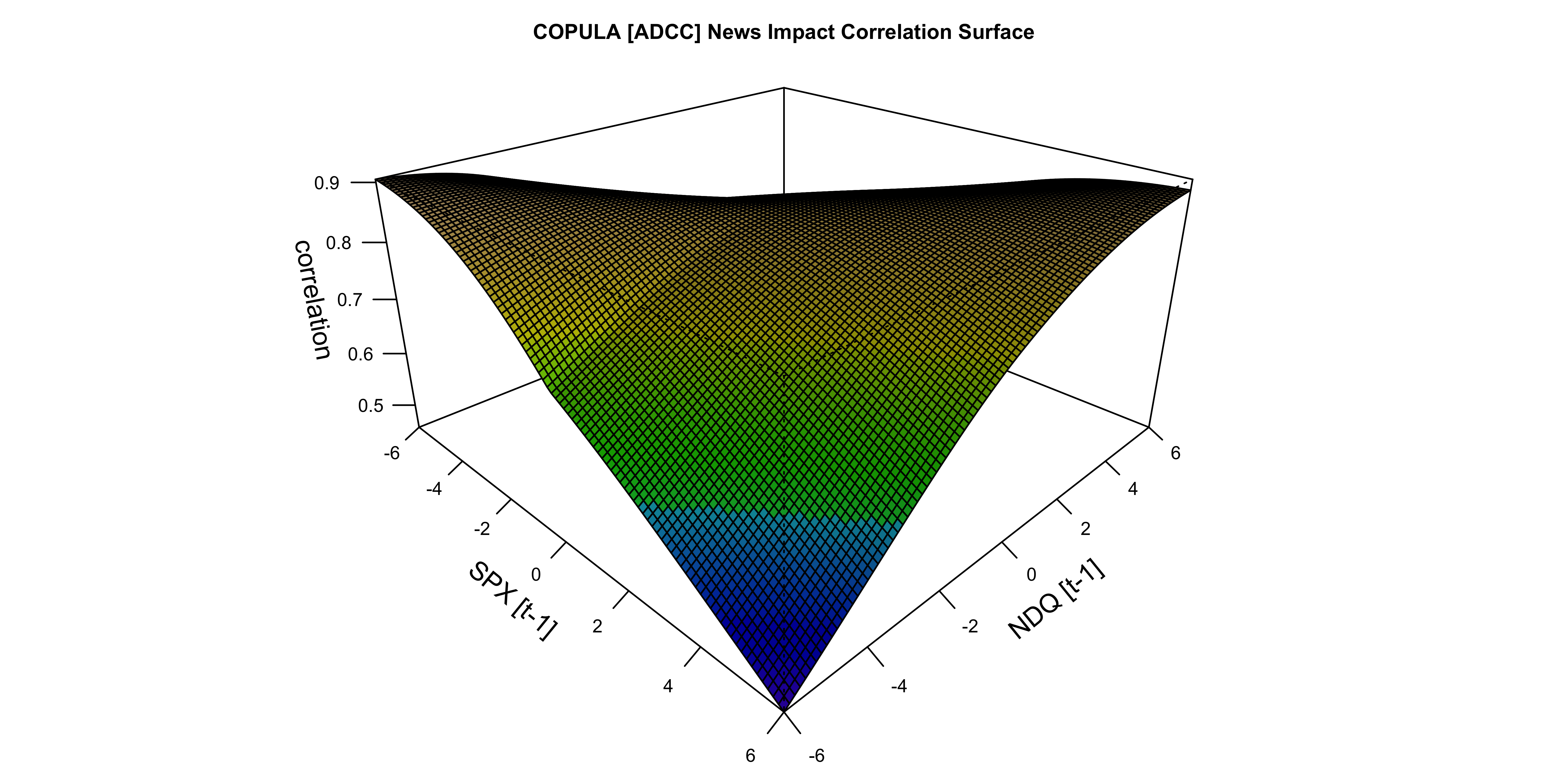
5.3.2 Prediction
The next step is to generate a rolling 1-step ahead forecast of the value at risk for the testing period similar to the approach we adopted for the DCC model:
Code
w <- rep(1/12, 12)
value_risk <- sapply(0:97, function(i){
  if (i == 0) {
    p <- cgarch_model |> predict(h = 1, nsim = 5000, seed = 100, cond_mean = .predicted[1,]) |> value_at_risk(weights = w, alpha = 0.05)
  } else {
    p <- cgarch_model |> tsfilter(y = .filtered_residuals[1:i,], cond_mean = .filtered_mean[1:i,]) |> predict(h = 1, cond_mean = .predicted[i + 1,], nsim = 5000, seed = 100) |> value_at_risk(weights = w, alpha = 0.05)
  }
  return(p)
})
value_risk <- xts(value_risk, index(test_set))
actual <- xts(coredata(test_set) %*% w, index(test_set))
as_flextable(var_cp_test(actual, value_risk, 0.05), signif.stars = TRUE, include.decision = TRUE)
Test | DoF | Statistic | Pr(>Chisq) | Decision(5%) | |
|---|---|---|---|---|---|
Kupiec (UC) | 1 | 2.3051 | 0.1290 | Fail to Reject H0 | |
CP (CCI) | 1 | 0.0842 | 0.7717 | Fail to Reject H0 | |
CP (CC) | 2 | 2.3893 | 0.3028 | Fail to Reject H0 | |
CP (D) | 1 | 4.0804 | 0.0434 | * | Reject H0 |
Signif. codes: 0 '***' 0.001 '**' 0.01 '*' 0.05 '.' 0.1 ' ' 1 | |||||
Coverage: 0.05, Obs: 98, Failures: 2, E[Failures]: 4 | |||||
Hypothesis(H0) : Unconditional(UC), Independent(CCI), Joint Coverage(CC) and Duration(D) | |||||
Similar to the DCC forecast, we reject the null for the conditional duration test.
We proceed to show the alternative way to predict, in this case for the long run forecast:
Code
p_1 <- cgarch_model |> predict(h = 98, nsim = 5000, seed = 100, cond_mean = .uncforecast)
# without centering, so that we get zero mean residuals
p_2 <- cgarch_model |> predict(h = 98, nsim = 5000, seed = 100)
simulated_res <- p_2$mu
arma_simulated_prediction <- lapply(1:12, function(i){
  tmp <- predict(cond_mean_model[[i]], h = 98, innov_type = "r", innov = t(simulated_res[,i,]), nsim = 5000, forc_dates = index(test_set))
  tmp <- tmp$distribution
  return(tmp)
})
and visually inspect the 2 approaches again:
Code
par(mfrow = c(2,1), mar = c(2,2,2,2))
plot(arma_simulated_prediction[[1]], main = "SPX Forecast Distribution",  gradient_color = "white")
cgarch_distribution <- t(p_1$mu[,1,])
colnames(cgarch_distribution) <- colnames(arma_simulated_prediction[[1]])
class(cgarch_distribution) <- "tsmodel.distribution"
plot(cgarch_distribution, add = TRUE, median_color = "red", gradient_color = "white", interval_color = "red")

plot(arma_simulated_prediction[[10]], main = "NKX Forecast Distribution", gradient_color = "white")
cgarch_distribution <- t(p_1$mu[,10,])
colnames(cgarch_distribution) <- colnames(arma_simulated_prediction[[10]])
class(cgarch_distribution) <- "tsmodel.distribution"
plot(cgarch_distribution, add = TRUE, median_color = "red", gradient_color = "white", interval_color = "red")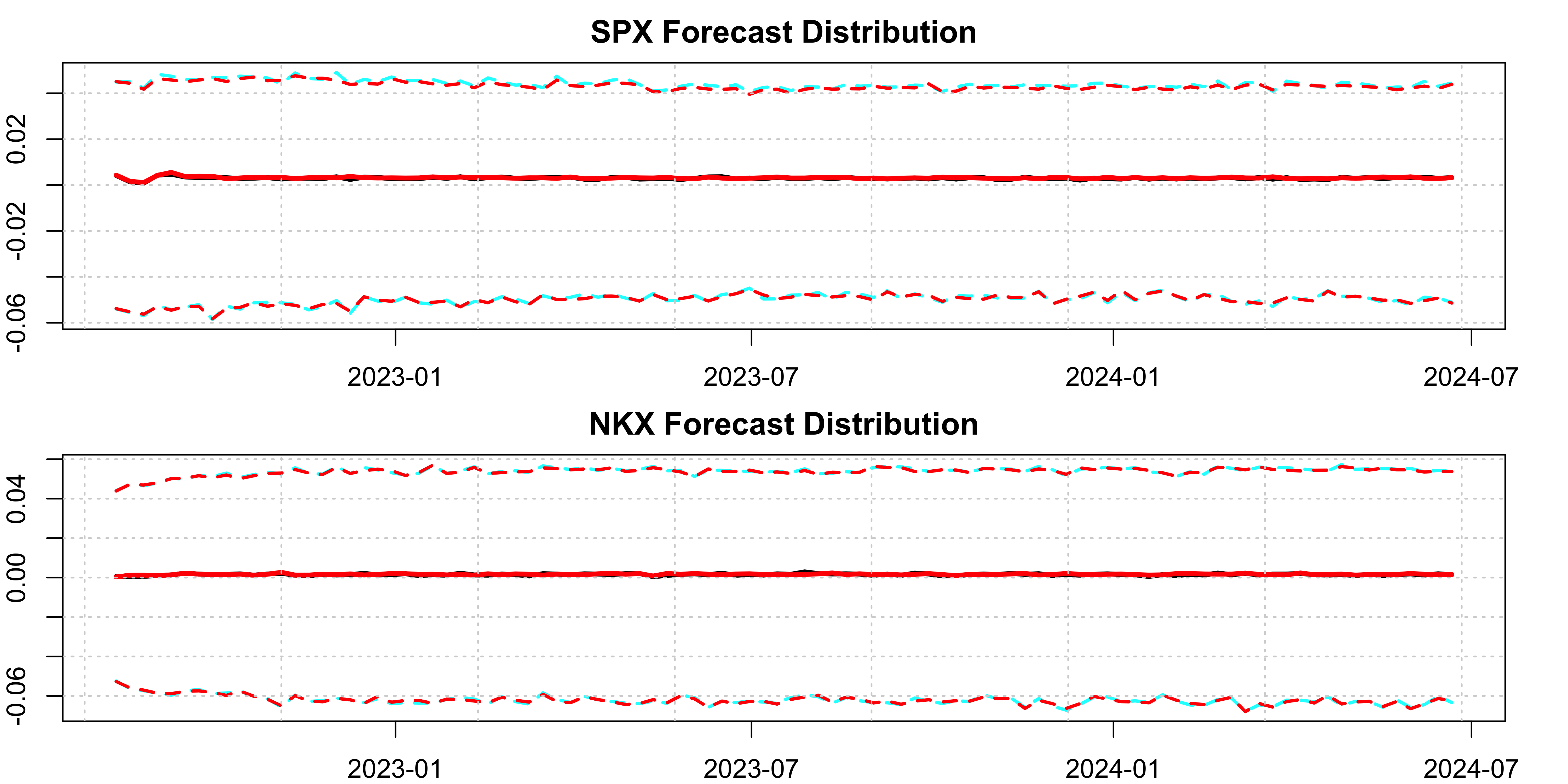
We can also form the value at risk of the weighted portfolio to check the correlation.
Code
# we re-center to the exact mean since we also do this for the DCC model distribution
arma_simulated_prediction <- lapply(1:12, function(i){
  d <- arma_simulated_prediction[[i]]
  d <- scale(d, scale = FALSE, center = TRUE)
  d <- scale(d, scale = FALSE, center = -as.numeric(.uncforecast[,i]))
  return(d)
})
arma_multi_correlated <- array(unlist(arma_simulated_prediction), dim = c(5000, 98, 12))
arma_multi_correlated <- aperm(arma_multi_correlated, perm = c(2, 3, 1))

v_1 <- do.call(cbind, lapply(1:98, function(i){
  t(arma_multi_correlated[i,,]) %*% w
}))
v_2 <- do.call(cbind, lapply(1:98, function(i){
  t(p_1$mu[i,,]) %*% w
}))
plot(apply(v_1, 2, quantile, 0.05), type = "l", ylab = "VaR 5%", xlab = "")
lines(apply(v_2, 2, quantile, 0.05), col = "orange", lty = 2, lwd = 2)
legend("topleft", c("ARMA Prediction with Copula-DCC correlated residuals","Copula-DCC Prediction with ARMA conditional mean recentering"), col = c("black","orange"), lty = c(1,2), lwd = c(1,2), bty = "n", cex = 0.8)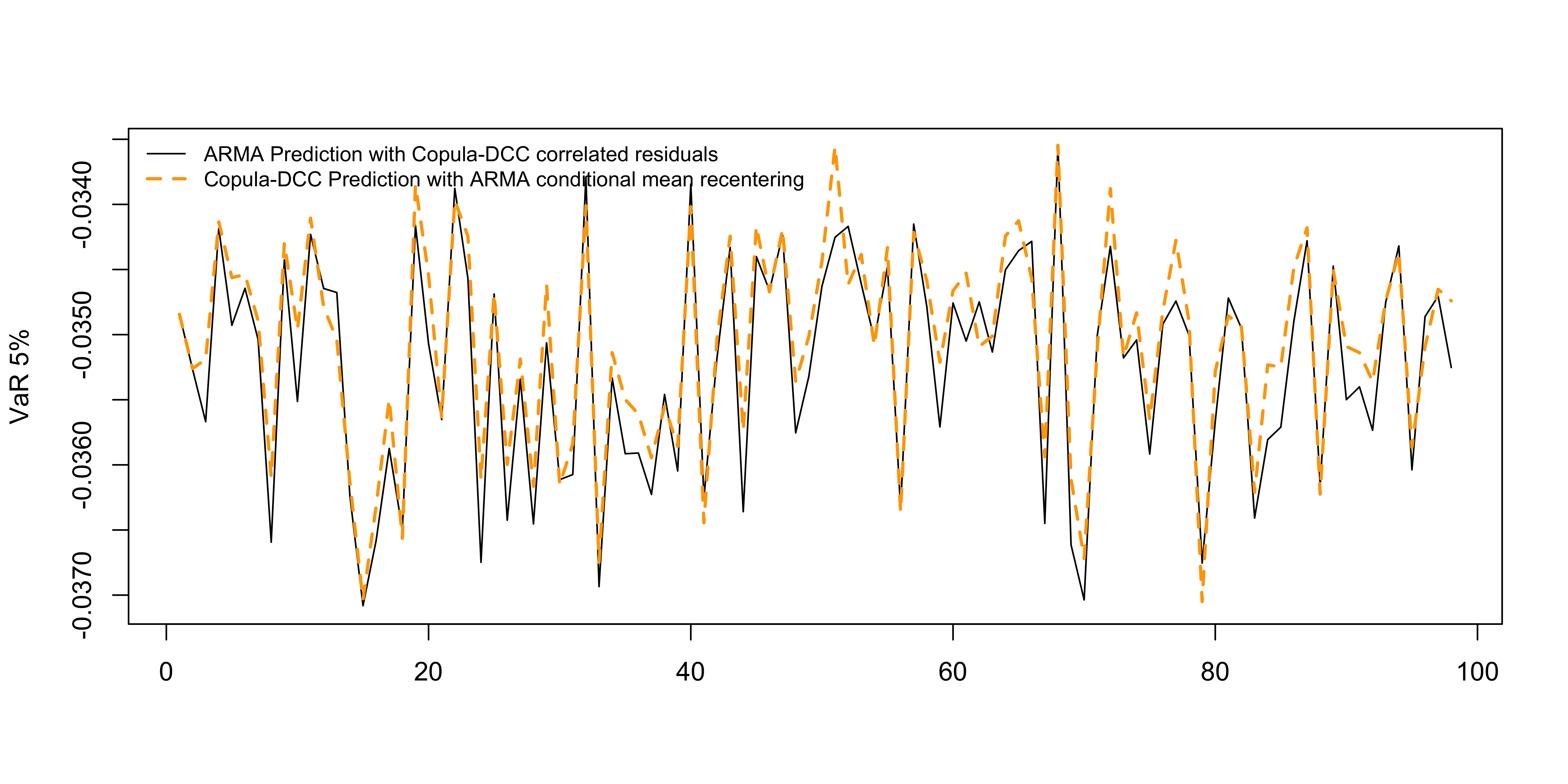
5.4 GOGARCH Model
5.4.1 Estimation
For the GOGARCH model we will make use of dimensionality reduction in the whitening (PCA) stage, extracting only the first 6 principal components.
Code
gogarch_model <- gogarch_modelspec(.residuals, model = "gjrgarch", distribution = "nig", components = 6, cond_mean = .fitted) |> estimate()The summary of GOGARCH model provides the univariate GARCH coefficients for the components as well as the rotation matrix U:
Code
summary(gogarch_model)## GOGARCH Model Summary
## Factor Dynamics: GJRGARCH | MANIG
## Coefficients:
## Estimate Std. Error t value Pr(>|t|)
## [IC_1]:omega 0.053228 0.010684 4.982 6.29e-07 ***
## [IC_1]:alpha1 0.242835 0.035526 6.835 8.18e-12 ***
## [IC_1]:gamma1 -0.218009 0.035863 -6.079 1.21e-09 ***
## [IC_1]:beta1 0.803103 0.027060 29.679 < 2e-16 ***
## [IC_1]:skew 0.408159 0.069392 5.882 4.05e-09 ***
## [IC_1]:shape 4.054943 1.146289 3.537 0.000404 ***
## [IC_1]:persistence 0.928761 0.017386 53.421 < 2e-16 ***
## [IC_2]:omega 0.002725 0.001513 1.801 0.071724 .
## [IC_2]:alpha1 0.075769 0.014306 5.296 1.18e-07 ***
## [IC_2]:gamma1 -0.038412 0.019134 -2.008 0.044689 *
## [IC_2]:beta1 0.940551 0.010345 90.920 < 2e-16 ***
## [IC_2]:skew 0.059431 0.050010 1.188 0.234687
## [IC_2]:shape 1.916958 0.449319 4.266 1.99e-05 ***
## [IC_2]:persistence 0.996831 0.004052 246.005 < 2e-16 ***
## [IC_3]:omega 0.008565 0.003428 2.499 0.012471 *
## [IC_3]:alpha1 0.090804 0.019745 4.599 4.25e-06 ***
## [IC_3]:gamma1 0.019147 0.026796 0.715 0.474901
## [IC_3]:beta1 0.893792 0.015584 57.353 < 2e-16 ***
## [IC_3]:skew -0.109429 0.049536 -2.209 0.027169 *
## [IC_3]:shape 2.343975 0.528024 4.439 9.03e-06 ***
## [IC_3]:persistence 0.993929 0.007566 131.362 < 2e-16 ***
## [IC_4]:omega 0.010819 0.004594 2.355 0.018530 *
## [IC_4]:alpha1 0.069125 0.013539 5.106 3.30e-07 ***
## [IC_4]:gamma1 -0.030525 0.018442 -1.655 0.097877 .
## [IC_4]:beta1 0.934654 0.012878 72.578 < 2e-16 ***
## [IC_4]:skew 0.147888 0.051076 2.895 0.003786 **
## [IC_4]:shape 2.961832 0.715934 4.137 3.52e-05 ***
## [IC_4]:persistence 0.988046 0.005916 166.999 < 2e-16 ***
## [IC_5]:omega 0.026241 0.007137 3.677 0.000236 ***
## [IC_5]:alpha1 0.137563 0.023548 5.842 5.16e-09 ***
## [IC_5]:gamma1 -0.086523 0.029338 -2.949 0.003186 **
## [IC_5]:beta1 0.874879 0.019649 44.525 < 2e-16 ***
## [IC_5]:skew 0.221667 0.052272 4.241 2.23e-05 ***
## [IC_5]:shape 2.268611 0.452716 5.011 5.41e-07 ***
## [IC_5]:persistence 0.966945 0.012574 76.902 < 2e-16 ***
## [IC_6]:omega 0.042102 0.012490 3.371 0.000749 ***
## [IC_6]:alpha1 0.156602 0.029468 5.314 1.07e-07 ***
## [IC_6]:gamma1 -0.094452 0.029411 -3.212 0.001320 **
## [IC_6]:beta1 0.850893 0.026374 32.262 < 2e-16 ***
## [IC_6]:skew 0.054504 0.052580 1.037 0.299925
## [IC_6]:shape 3.018993 0.812674 3.715 0.000203 ***
## [IC_6]:persistence 0.959735 0.015020 63.895 < 2e-16 ***
## ---
## Signif. codes: 0 '***' 0.001 '**' 0.01 '*' 0.05 '.' 0.1 ' ' 1
##
## Rotation Matrix (U):
## 0.888032 0.137009 0.022684 0.270669 0.316058 0.137692
## -0.235925 0.611359 -0.416872 0.608046 -0.134342 0.095028
## -0.158537 0.375395 0.864432 0.112464 0.005831 0.272065
## -0.022919 -0.609074 0.209544 0.713822 -0.241885 -0.128629
## -0.304091 -0.027647 0.039095 0.183043 0.862543 -0.357421
## -0.193928 -0.307917 -0.181723 0.036392 0.282022 0.868156
##
## N: 1600 | Series: 12 | Factors: 6
## LogLik: 11999.1, AIC: -23854.2, BIC: -23467The plot below shows the newsimpact correlation surface between a pair of series and factors (components):
Code
newsimpact(gogarch_model, pair = c(1,6), factor = c(1,6), type = "correlation") |> plot()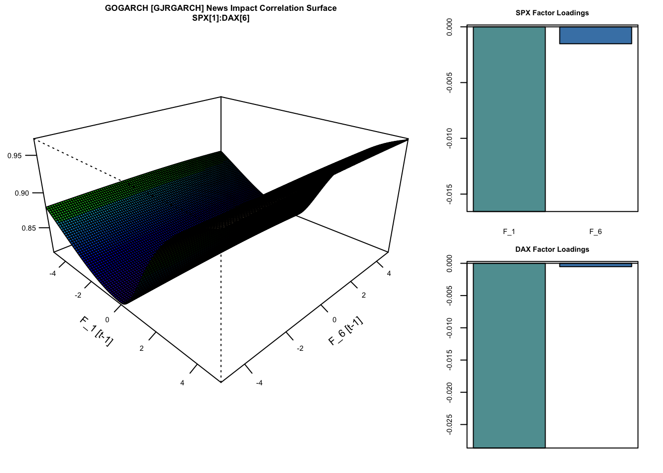
5.4.2 Prediction
We continue with a rolling 1-step ahead forecast of the value at risk for the testing period similar to the approach we adopted for the DCC model:
Code
w <- rep(1/12, 12)
value_risk <- sapply(0:97, function(i){
  if (i == 0) {
    p <- gogarch_model |> predict(h = 1, nsim = 5000, seed = 100, cond_mean = .predicted[1,]) |> value_at_risk(weights = w, alpha = 0.05)
  } else {
    p <- gogarch_model |> tsfilter(y = .filtered_residuals[1:i,], cond_mean = .filtered_mean[1:i,]) |> predict(h = 1, cond_mean = .predicted[i + 1,], nsim = 5000, seed = 100) |> value_at_risk(weights = w, alpha = 0.05)
  }
  return(p)
})
value_risk <- xts(value_risk, index(test_set))
actual <- xts(coredata(test_set) %*% w, index(test_set))
as_flextable(var_cp_test(actual, value_risk, 0.05), signif.stars = TRUE, include.decision = TRUE)
Test | DoF | Statistic | Pr(>Chisq) | Decision(5%) | |
|---|---|---|---|---|---|
Kupiec (UC) | 1 | 0.1851 | 0.6670 | Fail to Reject H0 | |
CP (CCI) | 1 | 0.3442 | 0.5574 | Fail to Reject H0 | |
CP (CC) | 2 | 0.5293 | 0.7675 | Fail to Reject H0 | |
CP (D) | 1 | 2.0525 | 0.1520 | Fail to Reject H0 | |
Signif. codes: 0 '***' 0.001 '**' 0.01 '*' 0.05 '.' 0.1 ' ' 1 | |||||
Coverage: 0.05, Obs: 98, Failures: 4, E[Failures]: 4 | |||||
Hypothesis(H0) : Unconditional(UC), Independent(CCI), Joint Coverage(CC) and Duration(D) | |||||
The GOGARCH model actually appears to perform much better that the DCC and CGARCH models, even in the presence of dimensionality reduction and we posit that this is due to the NIG margins which provide for a better fit to the actual data.
The next example uses the convolution approach to generate a 1-step ahead value at risk surface in order to highlight the functionality of this method:
Code
w <- rep(1/12, 12)
q_seq <- seq(0.025, 0.975, by = 0.025)
value_risk_surface <- do.call(rbind, lapply(0:97, function(i){
  if (i == 0) {
    fun <- gogarch_model |> predict(h = 1, nsim = 5000, seed = 100, cond_mean = .predicted[1,]) |> tsconvolve(distribution = FALSE, weights = w) |> qfft(index = 1)
    matrix(fun(q_seq), nrow = 1)
  } else {
    fun <- gogarch_model |> tsfilter(y = .filtered_residuals[1:i,], cond_mean = .filtered_mean[1:i,]) |> predict(h = 1, cond_mean = .predicted[i + 1,], nsim = 5000, seed = 100) |> tsconvolve(distribution = FALSE, weights = w) |> qfft(index = 1)
    matrix(fun(q_seq), nrow = 1)
  }
}))

par(mar = c(1.8,1.8,1.1,1), pty = "m")
col_palette <- drapecol(value_risk_surface, col = femmecol(100), NAcol = "white")
persp(x = 1:98, y = q_seq, z = value_risk_surface,  col = col_palette, theta = 45,
      phi = 15, expand = 0.5, ltheta = 25, shade = 0.25,
      ticktype = "simple", xlab = "Time", ylab = "Quantile",
      zlab = "VaR", cex.axis = 0.8, main = "Value at Risk Prediction Surface")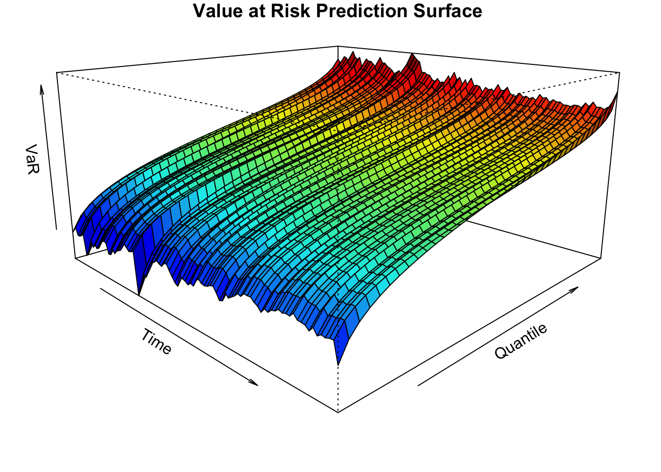
5.4.3 Co-Moments
The GOGARCH model uniquely generates higher co-moment matrices, from which closed form weighted higher moments may then be obtained using the tsaggregate method. This allows either a predictive distribution to be generated or the expected value (set by the distribution argument):
Code
p <- predict(gogarch_model, h = 98, cond_mean = .uncforecast)
gogarch_moments <- tsaggregate(p, weights = w, distribution = FALSE)
par(mfrow = c(2,2), mar = c(2,2,2,2))
plot(as.Date(p$forc_dates), as.numeric(gogarch_moments$mu), main = "Portfolio Mean", ylab = "", xlab = "", type = "l")
grid()
plot(as.Date(p$forc_dates), as.numeric(gogarch_moments$sigma), main = "Portfolio Sigma", ylab = "", xlab = "", type = "l")
grid()
plot(as.Date(p$forc_dates), as.numeric(gogarch_moments$skewness), main = "Portfolio Skewness", ylab = "", xlab = "", type = "l")
grid()
plot(as.Date(p$forc_dates), as.numeric(gogarch_moments$kurtosis), main = "Portfolio Kurtosis", ylab = "", xlab = "", type = "l")
grid()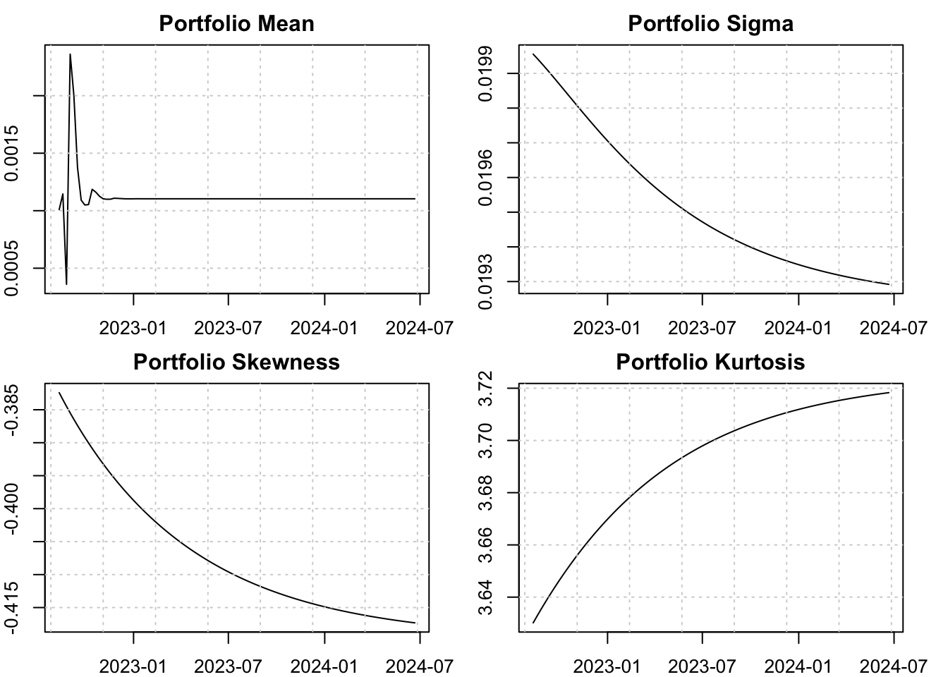
6 Not Implemented
The following are yet to be implemented and may be included in a future release:
- The test of Constant Correlation.
- A backtest method (
tsbacktest) for the models. - The indirect DCC model.
7 Appendix
7.1 Correlation and Kendall’s \(\tau\)
Pearson’s product moment correlation \(R\) totally characterizes the dependence structure in the multivariate Normal case, where zero correlation also implies independence, but can only characterize the ellipses of equal density when the distribution belongs to the elliptical class. In the latter case for instance, with a distribution such as the multivariate Student, the correlation cannot capture tail dependence determined by the shape parameter. Furthermore, it is not invariant under monotone transformations of original variables making it inadequate in many cases. An alternative measure which does not suffer from this is Kendall’s \(\tau\) (see Kruskal (1958)), based on rank correlations which makes no assumption about the marginal distributions but depends only on the Copula \(C\). It is a pairwise measure of concordance calculated as:
\[ \tau(x_i, x_j) = 4 \int_0^1 \int_0^1 C\left(u_i, u_j\right) \, dC\left(u_i, u_j\right) - 1 \tag{42}\]
For elliptical distributions, Lindskog, Mcneil, and Schmock (2003), proved that there is a one-to-one relationship between this measure and Pearson’s correlation coefficient \(\rho\) given by:
\[ \tau(x_i, x_j) = \left( 1 - \sum_{x \in \mathbb{R}} \left( \mathbb{P}\{X_i = x\}^2 \right) \right) \frac{2}{\pi} \arcsin \rho_{ij} \tag{43}\]
which under certain assumptions (e.g. in the multivariate Normal case) simplifies to \[\frac{2}{\pi} \arcsin \rho_{ij}\]. Kendall’s \(\tau\) is invariant under monotone transformations making it more suitable when working with non-elliptical distributions. A useful application arises in the case of the multivariate Student distribution where the maximum likelihood approach for the estimation of the correlation matrix \(R\) become unfeasible for large dimensions. Instead, estimating the sample counterpart of Kendall’s \(\tau\) from the transformed margins and then translating that into a correlation matrix as detailed in Equation 43 provides for a method of moments type estimator. The shape parameter \(\nu\) is then estimated keeping the correlation matrix constant, with little loss in efficiency.
7.2 Notes on Selected Methods
The table below provides a summary of selected methods, the classes they belong to, the classes they output, whether they are parallelized and the dimensions of the objects involved. For example, the tsaggrate method on predicted and simulated objects will return a list of length 4, with each slot having an object of class tsmodel.distribution of size \(sim\times h\) representing the predictive simulatated distribution of each of the weighted moments generated by the model.10 The output for the tsconvolve method which is list(h):list(sim) means that the output is a list of length \(h\) where each slot contains a list of length \(sim\).
| Method | class (in) | class (out) | future | RcppParallel | dimensions |
|---|---|---|---|---|---|
tscov |
(1,4,7) | matrix |
no | no | [n, n, T] |
tscov |
(2,3,5,6,8,9) | matrix |
no | no | [n, n, h, sim] |
tscoskew |
(1) | matrix |
no | yes | [n, n², T] |
tscoskew |
(2,3) | matrix |
no | yes | [n, n², h, sim] |
tscokurt |
(1) | matrix |
no | yes | [n, n³] |
tscokurt |
(2,3) | matrix |
no | yes | [n, n³, h, sim] |
tsconvolve |
(1) | gogarch.fft |
yes | no | list(T) |
tsconvolve |
(2,3) | gogarch.fftsim |
yes | no | list(h):list(sim) |
tsaggregate |
(1,4,7) | list |
no | yes | 4:n |
tsaggregate |
(2,3,5,6,8,9) | list |
no | yes | 4:(sim x h) |
Key for class (in):
- 1:
gogarch.estimate - 2:
gogarch.predict - 3:
gogarch.simulate - 4:
dcc.estimate - 5:
dcc.predict - 6:
dcc.simulate - 7:
cgarch.estimate - 8:
cgarch.predict - 9:
cgarch.simulate
7.3 References
Footnotes
This is relevant for the DCC type models and not the GOGARCH model which is based on independent components.↩︎
After considerable experimentation, it was chosen to avoid the use of automatic differentiation and instead use numerical derivatives for the second stage estimation due to speed considerations, and observing that there was little gain in terms of accuracy.↩︎
Technically, up to 1 component may be Gaussian.↩︎
To speed estimation, parts of the RADICAL algorithm are parallelized in C++ using
RcppParalleland hence benefits from multi-threading.↩︎When \(U\) is restricted to be an identity matrix, the model reduces to the Orthogonal Factor model.↩︎
Technically, the
nigdistribution is a special case of theghdistribution with \(\lambda = -0.5\), but since is possesses some nice properties, it is included as a separate distribution for speed purposes.↩︎The package allows to extract these tensors in both folded and unfolded form.↩︎
We loop through all possible combinations of shocks for factors k and l which were previously calculated from their respective news impact curves using a common grid of shock values \(\{\epsilon_1,\ldots,e_z\}\)↩︎
The
tsfiltermethod returns an updated object of the same class as theestimatemethod hence has an arrow going back to that method to denote this.↩︎For the DCC and Copula GARCH models only the first 2 moments are time varying and hence contain a simulated distribution.↩︎